Chapter 15 Univariate Analysis
15.1 Measurement Scales
We have two kinds of variables:
Qualitative, or Attribute, or Categorical, Variable: A variable that categorizes or describes an element of a population. Note: Arithmetic operations, such as addition and averaging, are not meaningful for data resulting from a qualitative variable.
Quantitative, or Numerical, Variable: A variable that quantifies an element of a population. Note: Arithmetic operations such as addition and averaging, are meaningful for data resulting from a quantitative variable.
Qualitative and quantitative variables may be further subdivided:
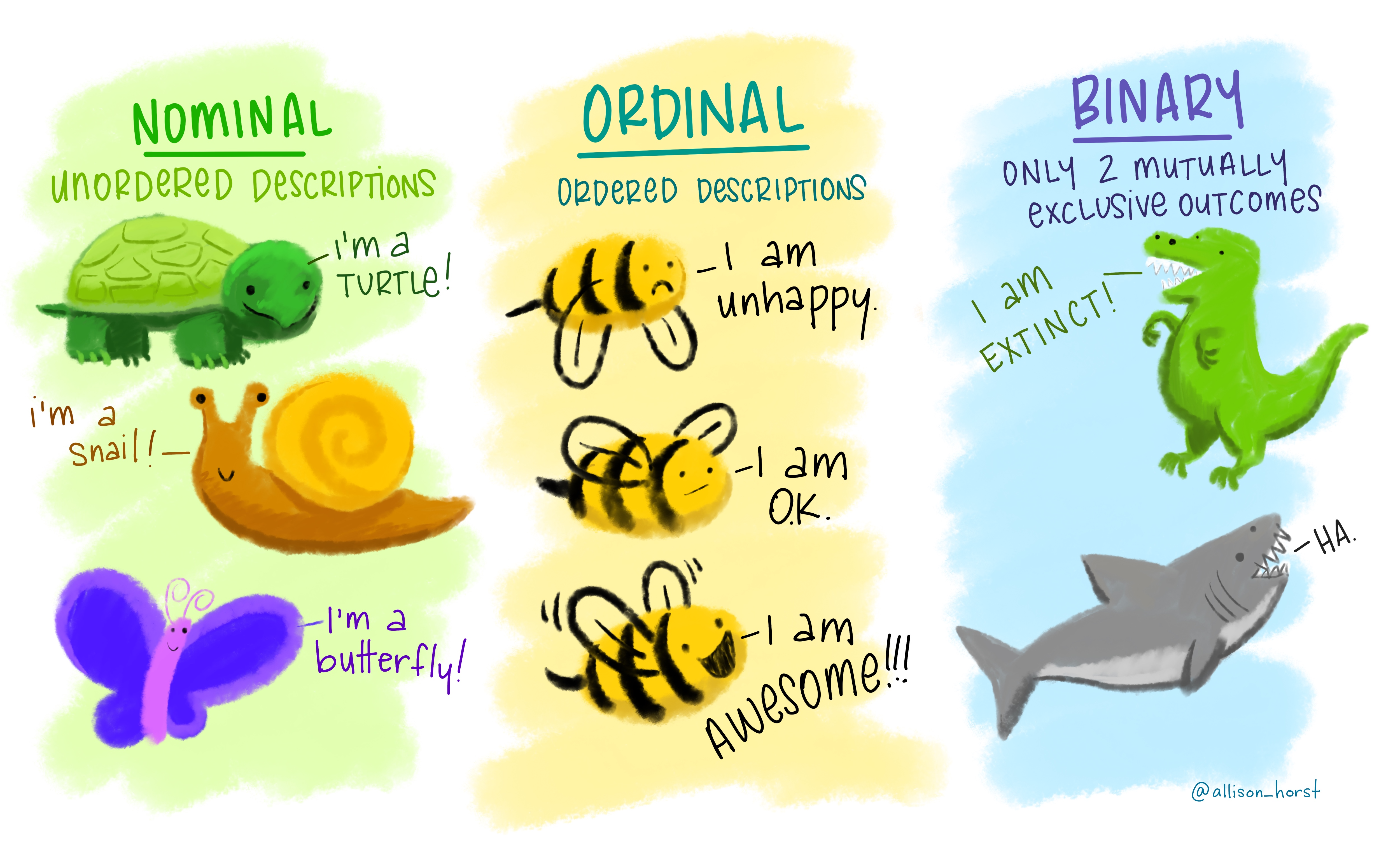
Nominal Variable: A qualitative variable that categorizes (or describes, or names) an element of a population.
Ordinal Variable: A qualitative variable that incorporates an ordered position, or ranking.
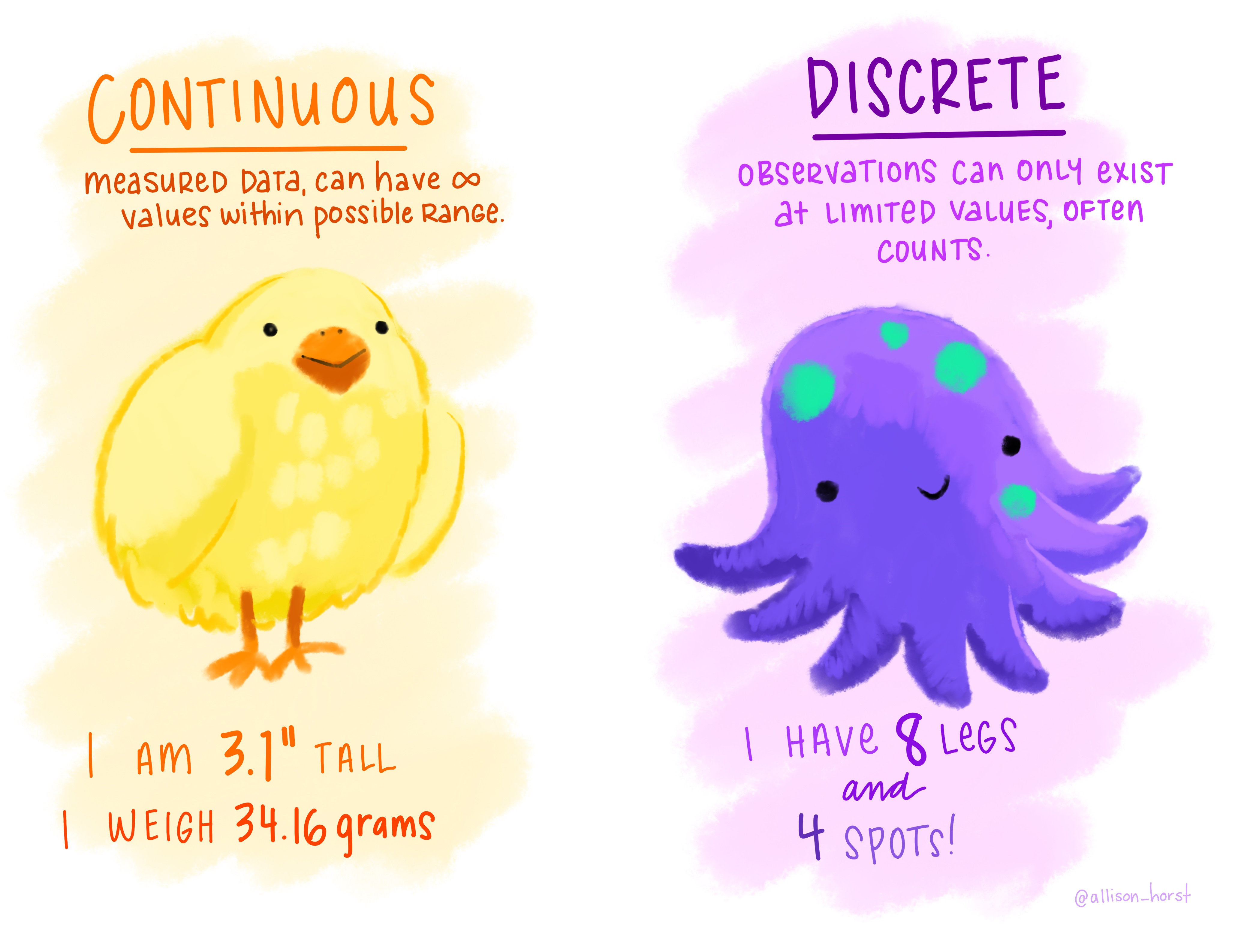
Discrete Variable: A quantitative variable that can assume a countable number of values. Intuitively, a discrete variable can assume values corresponding to isolated points along a line interval. That is, there is a gap between any two values. One example: binary variable (0-1).
Continuous Variable: A quantitative variable that can assume an uncountable number of values. Intuitively, a continuous variable can assume any value along a line interval, including every possible value between any two values.
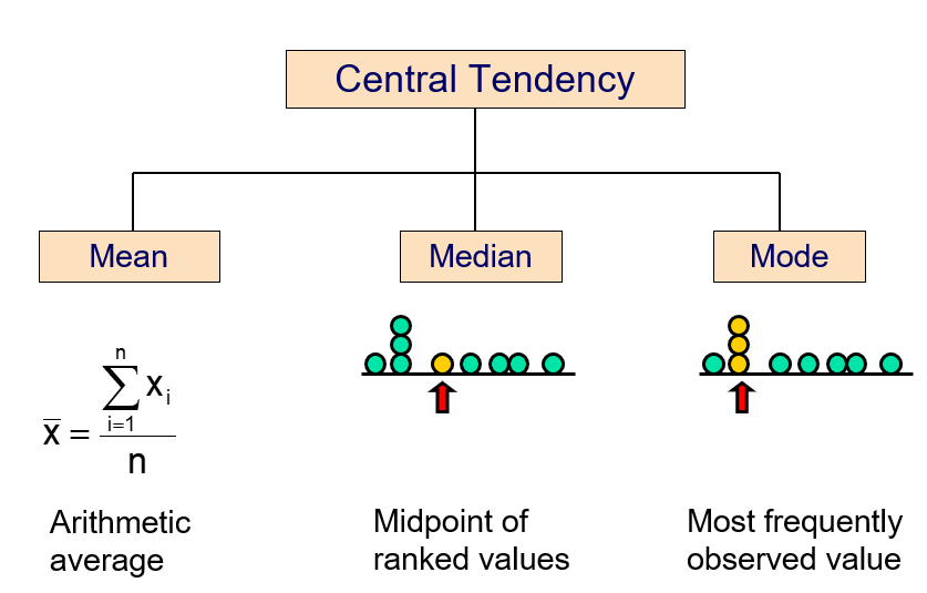
15.2 Central Tendency
We can use many different statistics to describe the central tendency of a given distribution.
15.2.1 Arithmetic mean
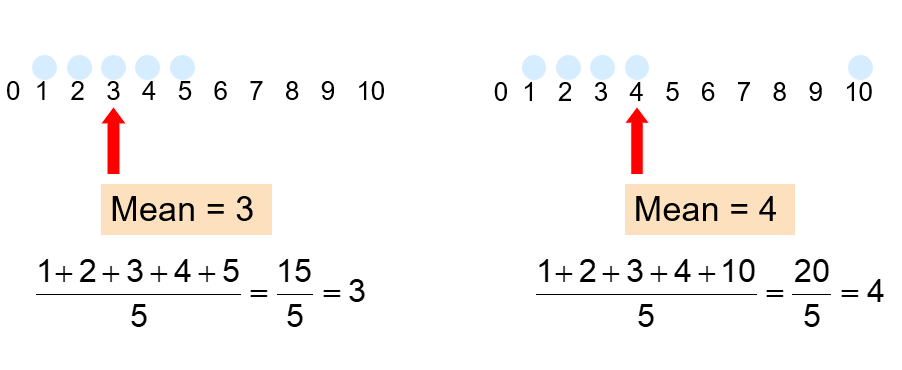
The arithmetic mean (mean) is the most common measure of central tendency.
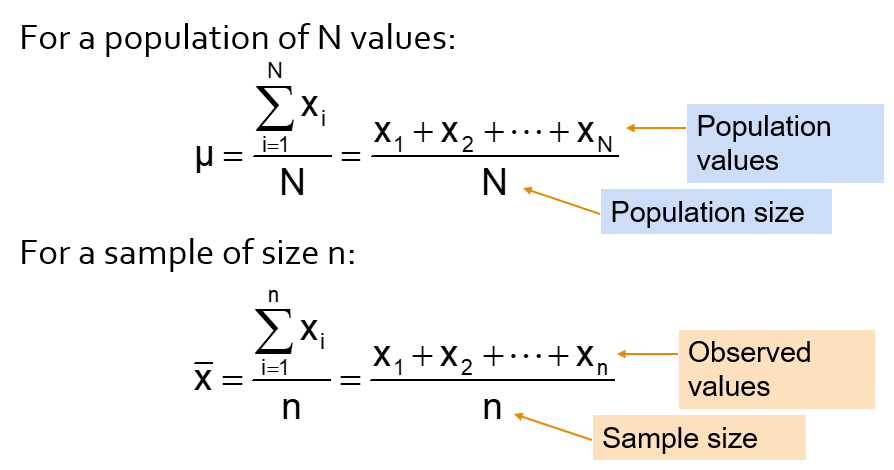
Mean = sum of values divided by the number of values, but unfortunately it is easily affected by extreme values (outliers).
- It requires at least the interval scale.
- All values are used
- It is unique
- It is easy to calculate and allow easy mathematical treatment
- The sum of the deviations from the mean is 0
- The arithmetic mean is the only measure of central tendency where the sum of the deviations of each value from the mean is zero!
- It is easily affected by extremes, such as very big or small numbers in the set (non-robust)
- For data stored in frequency tables use weighted mean!
Let’s calculate the mean for miles per gallon variable (“mtcars” data):
mean(mtcars$mpg)## [1] 20.0906215.2.2 Median
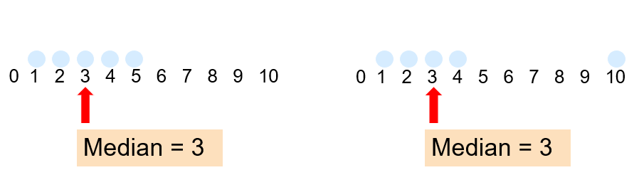
In an ordered list, the median is the “middle” number (50% above, 50% below).
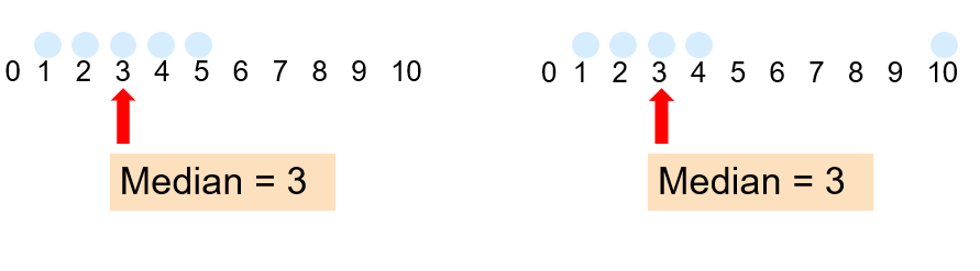
Not affected by extreme values!
- It requires at least the ordinal scale
- All values are used
- It is unique
- It is easy to calculate but does not allow easy mathematical treatment
- It is not affected by extremely large or small numbers (robust)!
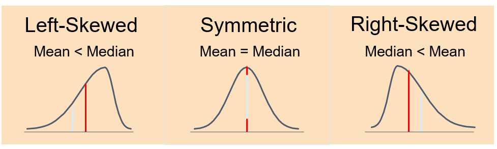
Median and mean may describe how data are distributed. Their comparison may witness of shape = if it is symmetric or skewed:
Median of mpg will be:
median(mtcars$mpg)## [1] 19.215.2.3 Mode
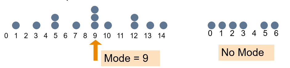
Mode is a measure of central tendency = the value that occurs most often. It is not affected by extreme values!
Usually used for either numerical or categorical data!
There may may be no mode!
There may be several modes!!
Mode function is included in “DescTools” library (not in Base R):
library("DescTools")
Mode(mtcars$mpg)
## [1] 10.4 15.2 19.2 21.0 21.4 22.8 30.4
## attr(,"freq")
## [1] 215.2.4 Quantiles
Quantiles are values that split sorted data or a probability distribution into equal parts. In general terms, a q-quantile divides sorted data into q parts. The most commonly used quantiles have special names:
- Quartiles (4-quantiles): Three quartiles split the data into four parts.
- Deciles (10-quantiles): Nine deciles split the data into 10 parts.
- Percentiles (100-quantiles): 99 percentiles split the data into 100 parts.
There is always one fewer quantile than there are parts created by the quantiles.
15.2.4.1 Quartiles
Quartiles split the ranked data into 4 segments with an equal number of values per segment:
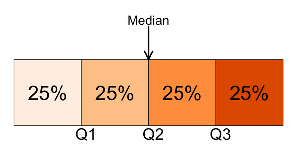
The first quartile, Q1, is the value for which 25% of the observations are smaller and 75% are larger. Q2 is the same as the median (50% are smaller, 50% are larger). Only 25% of the observations are greater than the third quartile!
Let’s calculate quartile for mpg variable using quantile function:
quantile(mtcars$mpg)## 0% 25% 50% 75% 100%
## 10.400 15.425 19.200 22.800 33.90015.2.4.2 Deciles
Further division of a distribution into a number of equal parts is sometimes used; the most common of these are deciles, percentiles, and fractiles.
Deciles divide the sorted data into 10 sections.
Now, let’s calculate all deciles for the mpg variable:
quantile(mtcars$mpg, probs=seq(0,1,0.1))## 0% 10% 20% 30% 40% 50% 60% 70% 80% 90% 100%
## 10.40 14.34 15.20 15.98 17.92 19.20 21.00 21.47 24.08 30.09 33.9015.3 Dispersion

Measures of variation give us information on the spread - dispersion or variability of the data values.
We can have the same center but different variation!
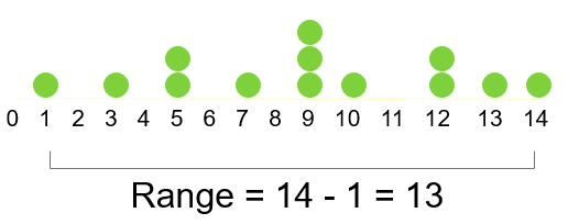
15.3.1 Range
Range is the simplest measure of variation.
Difference between the largest and the smallest observations:

Example:
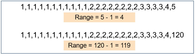
 Range ignores the way in which data are distributed and is very sensitive to outliers:
Let’s calculate range for mpg variable:
range(mtcars$mpg)## [1] 10.4 33.915.3.2 Interquartile range
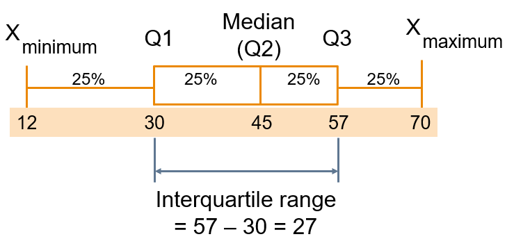
We can eliminate some outlier problems by using the interquartile range. We may eliminate high- and low- valued observations and calculate the range of the middle 50% of the data.
Interquartile range = 3rd quartile – 1st quartile
 Let’s calculate iqr range for mpg variable:
IQR(mtcars$mpg)## [1] 7.37515.3.3 Variance
Variance is the measure of spread. It is the average of squared deviations of values from the mean:
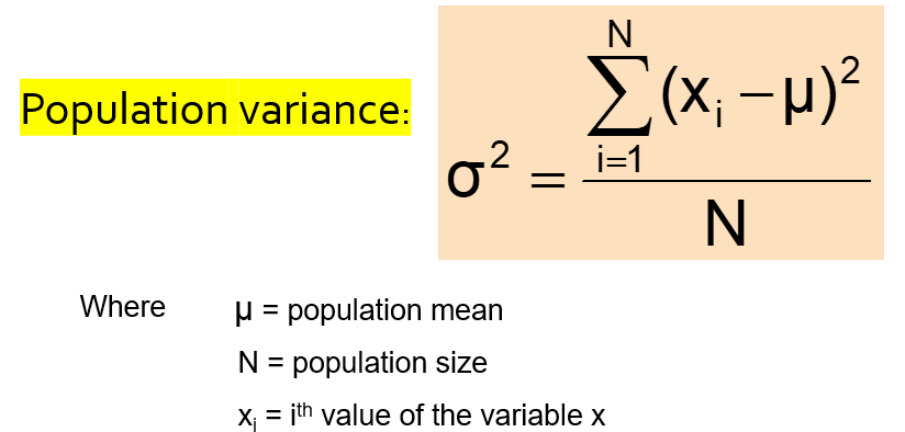
Sample variance is the average (approximately) of squared deviations of values from the mean:
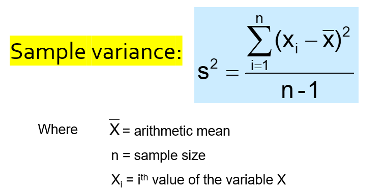
Let’s calculate the sample variance for mpg variable:
var(mtcars$mpg)## [1] 36.3241It cannot be interpreted (squared units - deviations from the mean) - so we must use square root of it.
15.3.4 Standard deviation
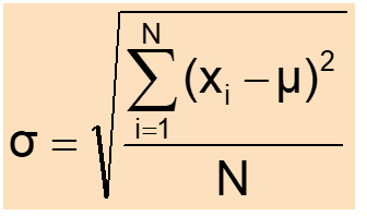
Standard deviation is the most commonly used measure of variation. It shows variation about the mean and has the same units as the original data.
Population standard deviation:
Sample standard deviation:
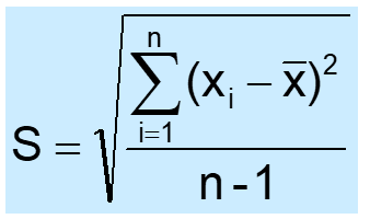
It is a measure of the “average” scatter around the mean.
Let’s compare several standard deviations:
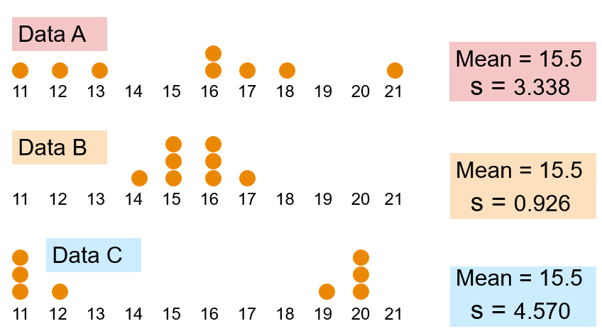 Any conclusions?
Each value in the data set is used in the calculation!
Values far from the mean are given extra weight (because deviations from the mean are squared).
Now, let’s calculate the standard deviation of the mpg distribution:
sd(mtcars$mpg)## [1] 6.02694815.3.5 % Variability
Many times it is easier to interpret volatility by simply converting the standard deviation into the percentage (relative) spread around the mean.
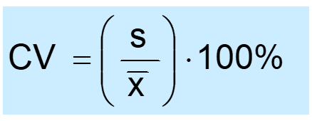
The coefficient of variability measures relative variation.
It can be used to compare two or more sets of data measured in different units.
The formula for CV:
Let’s write our own function to calculate it for mpg variable:
cv <- function(variable) { sd (variable) / mean (variable) }
cv(mtcars$mpg)
## [1] 0.2999881We have 29.99% of variability in mpg distribution (quite low) - the mean mpg is almost 30% of its variation.
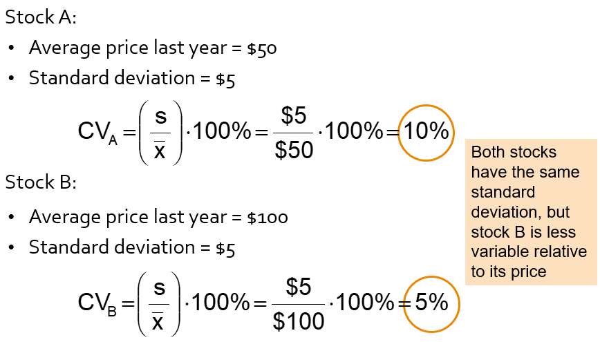
CV may be useful for comparing variability in 2 or more distributions:
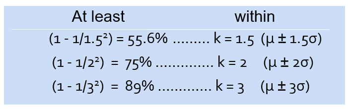
15.4 Chebychev’s rule
For any population with mean μ and standard deviation σ, and k > 1, the percentage of observations that fall within the interval:
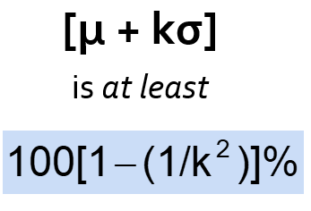
Regardless of how the data are distributed, at least (1 - 1/k2) of thevalues will fall within k standard deviations of the mean (for k > 1)
Examples:
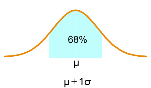
15.5 Empirical rule
If the data distribution is bell-shaped, then the interval:
- range of 1 standard deviation around the mean contains about 68% of the values in the population or the sample
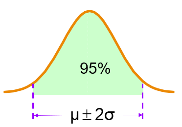
- range of 2 standard deviations around the mean contains about 95% of the values in the population or the sample
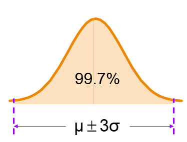
- range of 3 standard deviations around the mean contains almost all (about 99.7%) of the values in the population or the sample
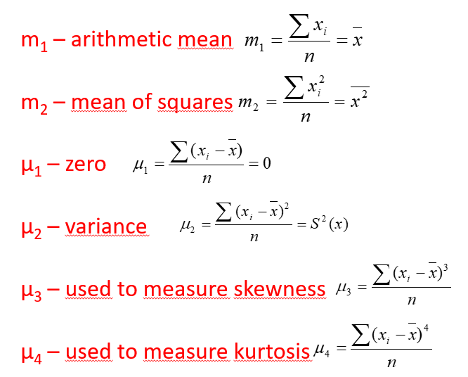
15.6 Method of moments
There are further statistics that describe the shape of the distribution, using formulas that are similar to those of the mean and variance - 1st moment - Mean (describes central value) - 2nd moment - Variance (describes dispersion) - 3rd moment - Skewness (describes asymmetry) - 4th moment - Kurtosis (describes tailedness)
The method of moments is a way to estimate population parameters, like the population mean or the population standard deviation.
The basic idea is that you take known facts about the population, and extend those ideas to a sample to capture its characteristics.
15.7 Skewness
While measures of dispersion are useful for helping us describe the width of the distribution, they tell us nothing about the shape of the distribution.
Skewness measures the degree of asymmetry exhibited by the data (normalized 3rd central moment):
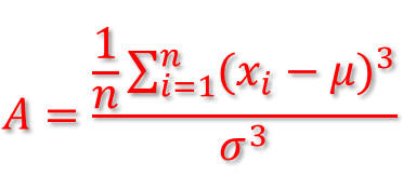
If skewness equals zero, the histogram is symmetric about the mean!
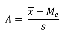
Pearson’s skewness coefficient:
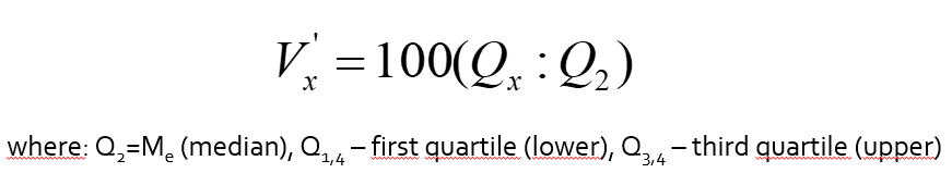
IQR Skewness measures the degree of asymmetry exhibited by the data between quartiles (around median):
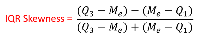
If IQR skewness equals zero, observations around median are equally distributed!
Positive skewness = there are more observations below the mean than above it; when the mean is greater than the median.
Negative skewness = there are a small number of low observations and a large number of high ones; when the median is greater than the mean.
Suppose we have the following dataset:
data = c(88, 95, 92, 97, 96, 97, 94, 86, 91, 95, 97, 88, 85, 76, 68)
hist(data, col='steelblue')
From the histogram we can see that the distribution appears to be left-skewed. That is, more of the values are concentrated on the right side of the distribution.
To calculate the skewness of this dataset, we can use skewness():
library(moments)
skewness(data)
## [1] -1.391777The skewness turns out to be -1.391777. Since the skewness is negative, this indicates that the distribution is left-skewed. This confirms what we saw in the histogram.
15.7.1 Skewness risk
Skewness risk is the risk that results when observations are not spread symmetrically around an average value, but instead have a skewed distribution.
As a result, the mean and the median can be different!
Skewness risk can arise in any quantitative model that assumes a symmetric distribution (such as the normal distribution) but is applied to skewed data.
Ignoring skewness risk, by assuming that variables are symmetrically distributed when they are not, will cause any model to understate the risk of variables with high skewness.
15.8 Kurtosis
Kurtosis measures the level of tailedeness.
It is a normalized 4th central moment:
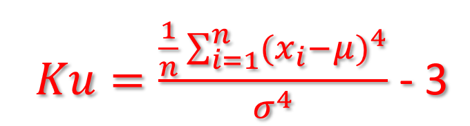
The kurtosis of a normal distribution is = 0.
Contrary to what is stated in some textbooks, kurtosis does not measure “flattening”, “peakedeness” of a distribution.
Kurtosis is influenced by the intensity of the extremes, so it measures what is happening in the “tails” of the distribution, the shape of the “tip” does not matter at all!
Platykurtic – When the kurtosis < 0, kurtosis is negative, the intensity of the extremes is less than that of the normal distribution (“narrower tails” of the distribution).
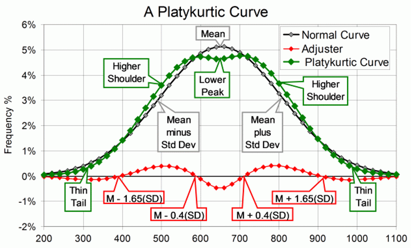
Short tails and a peak flattened to form a broad back!
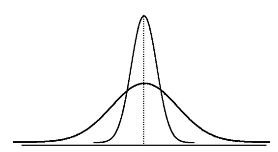
Leptokurtic – When the kurtosis > 0, the kurtosis is positive, the intensity of the extreme values is greater than for the normal distribution (the “tails” of the distribution are “thicker”).
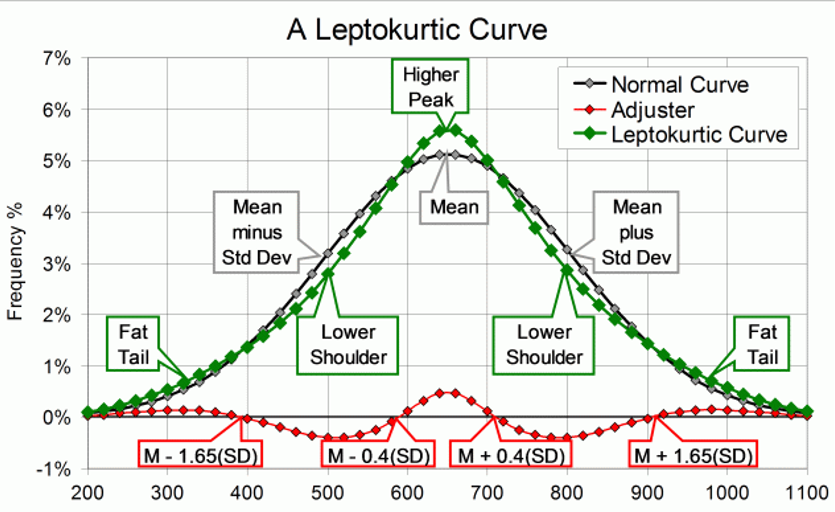
By adding the “adjuster curve” (red) to the Normal curve, we get the classical leptokurtic shape (green). It has a higher peak, lowered shoulders, and fat tails. The shape is like that of a volcanic cone: the peak is narrow, and the upper slopes steep. The slopes get gentler as they get lower, but not as gentle as on the Normal Curve.
Let’s calculate kurtosis for our simple dataset:
library(moments)
data = c(88, 95, 92, 97, 96, 97, 94, 86, 91, 95, 97, 88, 85, 76, 68)
hist(data, col='steelblue')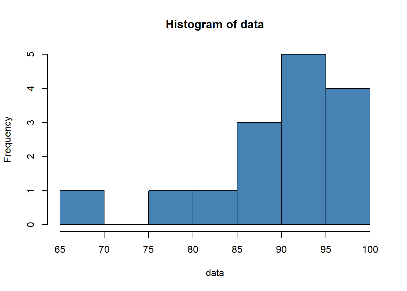
kurtosis(data)## [1] 4.177865The kurtosis turns out to be 4.177865. Since the kurtosis is greater than 3, this indicates that the distribution has more values in the tails compared to a normal distribution.
Kurtosis is based on the size of a distribution’s tails.
Negative kurtosis (platykurtic) – distributions with short tails!
Positive kurtosis (leptokurtic) – distributions with relatively long tails!
Medium kurtosis (mesokurtic) - gaussian!
Why Do We Need Kurtosis?
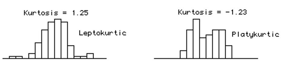
These two distributions have the same variance, approximately the same skew, but differ markedly in kurtosis!
15.8.1 Kurtosis risk
Kurtosis risk is the risk that results when a statistical model assumes the normal distribution, but is applied to observations that do not cluster as much near the average but rather have more of a tendency to populate the extremes either far above or far below the average
Kurtosis risk is commonly referred to as “fat tail” risk. The “fat tail” metaphor explicitly describes the situation of having more observations at either extreme than the tails of the normal distribution would suggest; therefore, the tails are “fatter”
Ignoring kurtosis risk will cause any model to understate the risk of variables with high kurtosis
15.9 Robust Statistics
In the case of outliers, traditional descriptive analysis may lead to erroneous conclusions. It is recommended to compare traditional results with the results of the so-called robust statistics.
15.9.1 Trimmed mean
Trimmed mean is next to the mean, mode and median - one of the statistical measures of central tendency. When calculating the trimmed mean, the observations are ordered from the smallest to the largest, the small percentage of the most extreme observations at both ends is rejected (the smallest and largest values in the sample), generally equal in size, and then the average of the remaining observations is calculated.
In general, the minimum and maximum of the sample or values below 25 percentile and above 75 percentile are rejected. This measure is an estimator that is not very sensitive to outliers. The extreme version of the trimmed mean, with the removal of a high percentage of observations in equal numbers from each end, is the median. This measure is used to calculate the points in figure skating competitions on ice and in other competitions in which points are awarded by a larger number of judges.
Now, let’s calculate the standard deviation of the mpg distribution trimming 10% on both ends:
mean(mtcars$mpg, trim=0.1)## [1] 19.6961515.9.2 Winsorized mean
Winsorized mean, often mistakenly called the “windsor mean” :) is one of averages, statistical measure of central tendency close to the usual arithmetic mean or median, and the most similar to the trimmed mean. It is calculated in the same way as the arithmetic mean, replacing the previously selected extreme observations (the predetermined number of the smallest and largest values in the sample) with the maximum and minimum values from the remaining part.
This procedure is sometimes called winsorisation. This name (and the name of the average) comes from the surname of the statistician Charles Winsor (1895-1951).
Typically, 10 to 25 percent of the range from both ends of the distribution is replaced. In the case when the coefficient is 0 percent, the Winsor average is reduced to the arithmetic mean, when all observations are replaced with the exception of one or two, it comes down to the median.
Winsorized mean is more robust to outliers than the arithmetic mean and even more robust than median to asymmetrical distribution of the variable.
The winsorized mean is less than the median resistant to outliers and less resistant than the arithmetic mean to the asymmetric distribution of the variable. It is an example of a robust estimate of the arithmetic mean in the population. However, with asymmetrical distributions, this is not an unbalanced estimator. An additional disadvantage, compared to the trimmed mean, is the large weight with which errors of estimation fall into the errors of two observations, the values of which are replaced by outliers.
Now, let’s calculate the winsorized mean and standard deviation of the mpg distribution:
library(psych)
winsor.mean(mtcars$mpg, trim = 0.2, na.rm = TRUE)
## [1] 19.3675winsor.sd(mtcars$mpg, trim = 0.2, na.rm = TRUE) ## [1] 3.508253winsor.var(mtcars$mpg, trim = 0.2, na.rm = TRUE) ## [1] 12.3078415.9.3 Trimmed sd
Among the robust estimates of central tendency are trimmed means and Winsorized means. The trimmed standard deviation is defined as the average trimmed sum of squared deviations around the trimmed mean.
Let’s calculate the trimmed (20% of data) mean and standard deviation of the mpg distribution:
library(chemometrics)
mean(mtcars$mpg, trim = 0.2)
## [1] 19.22sd_trim(mtcars$mpg, trim = 0.2) ## [1] 5.192485Rather than just dropping the top and bottom trim percent, these extreme values are replaced with values at the trim and 1- trim quantiles. We used trim = 20% of data to moved from the top and bottom of the mpg distribution.
15.9.4 MAD
The median absolute deviation (MAD), i.e., the (lo-/hi-) median of the absolute deviations from the median, and (by default) adjust by a factor for asymptotically normal consistency.
Median spread - Median Absolute Deviation - MAD:
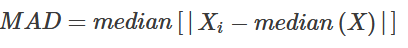
This statistics is more resistant to atypical observations than the classic standard deviation (note: there exists of course “trimmed standard deviation” measure too). In standard deviation, the distances (distances) of each observation from the mean are raised to a square, so long distances affect its result more than smaller - that is, outliers very much fall into results. MAD is insensitive to these deviations.
It is proved that:
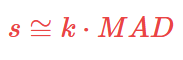
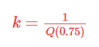
Scaling coefficient k for asymmetrical distributions is equal to 1,4826. For other distributions this factor must be calculated based on the formula:
 Now, let’s calculate the MAD of the mpg distribution:
mad(mtcars$mpg, na.rm = TRUE)## [1] 5.41149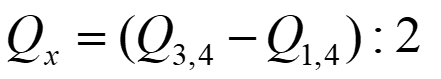
15.10 Summary reports
Using kableextra package we can easily create summary tables with graphics and/or statistics.
##
## Dołączanie pakietu: 'kableExtra'
## Następujący obiekt został zakryty z 'package:dplyr':
##
## group_rows| cyl | boxplot | histogram | line1 | line2 | points1 |
|---|---|---|---|---|---|
| 4 | |||||
| 6 | |||||
| 8 |
We can finally summarize basic measures for mpg variable by number of cylinders using ‘kable’ package. You can customize your final report. See some hints here.
| 4 cylinders | 6 cylinders | 8 cylinders | |
|---|---|---|---|
| Min | 10.40 | 10.40 | 10.40 |
| Max | 33.90 | 33.90 | 33.90 |
| Q1 | 15.43 | 15.43 | 15.43 |
| Median | 19.20 | 19.20 | 19.20 |
| Q3 | 22.80 | 22.80 | 22.80 |
| Mean | 20.09 | 20.09 | 20.09 |
| Sd | 6.03 | 6.03 | 6.03 |
| IQR | 7.38 | 7.38 | 7.38 |
| Sx | 3.69 | 3.69 | 3.69 |
| Var % | 0.30 | 0.30 | 0.30 |
| IQR Var % | 0.38 | 0.38 | 0.38 |
| Skewness | 0.61 | 0.61 | 0.61 |
| Kurtosis | -0.37 | -0.37 | -0.37 |