Chapter 17 Simple Regression

17.1 OLS approach

The Ordinary Least Squares (OLS) estimators for coefficients $\widehat{\beta}_0$ and $\widehat{\beta}_1$ are those that minimize the squared sum of residuals produced by those estimators, that is

\[\text{Find}~~(\widehat{\beta}_0, \widehat{\beta}_1) \text{ such that } \sum^n_{i = 1}(y_i - \hat{u}_i)^2 \text{is minimized} \]

In math, we use the symbol $\text{argmin}_{b_0, b_1}$ to indicate the same thing, the values such that…

\[(\widehat{\beta}_0, \widehat{\beta}_1) = \arg\min_{b_0, b_1}\sum^n_{i-1}(y_i - (b_0 + b_1 x_i))^2 \]

Why do we square the residuals? We need some way to have the errors add up, not cancel out. Why not use absolute values instead? The short answer here is that using squares makes minimization much easier to work with. Minimization requires derivatives, and taking a derivative of a square is more straightforward than trying to take a derivative of an absolute value. Also, when we use squared error we obtain familiar terms such as covariance and variance in our estimation.

Doing the math of taking the derivative of $(y_i - (\widehat{\beta}_0 + \widehat{\beta}_1 x_i))^2$ and setting it to zero, we get the following formula.

The Slope Coefficient for Simple Regression

The OLS estimator for the slope coefficient is \[\widehat{\beta}_1 = \frac{\widehat{\cov}(X, y)}{\widehat{\var}(X)}\]

We can also re-express this in terms of sums of squares because sample covariance and sample variance have the same denominator.

\[\begin{align*} \widehat{\beta}_1 &= \frac{\widehat{\cov}(X, y)}{\widehat{\var}(X)}\\ &= \frac{\frac{1}{n-1}\sum^n_{i=1}(x_i - \bar{x})(y_i - \bar{y})}{\frac{1}{n-1}\sum^n_{i=1}(x_i - \bar{x})^2}\\ &= \frac{\sum^n_{i=1}(x_i - \bar{x})(y_i - \bar{y})}{\sum^n_{i=1}(x_i - \bar{x})^2} \end{align*}\]

17.2 Linear regression

The linear model is arguably the most widely used statistical model, has a place in nearly every application domain of statistics

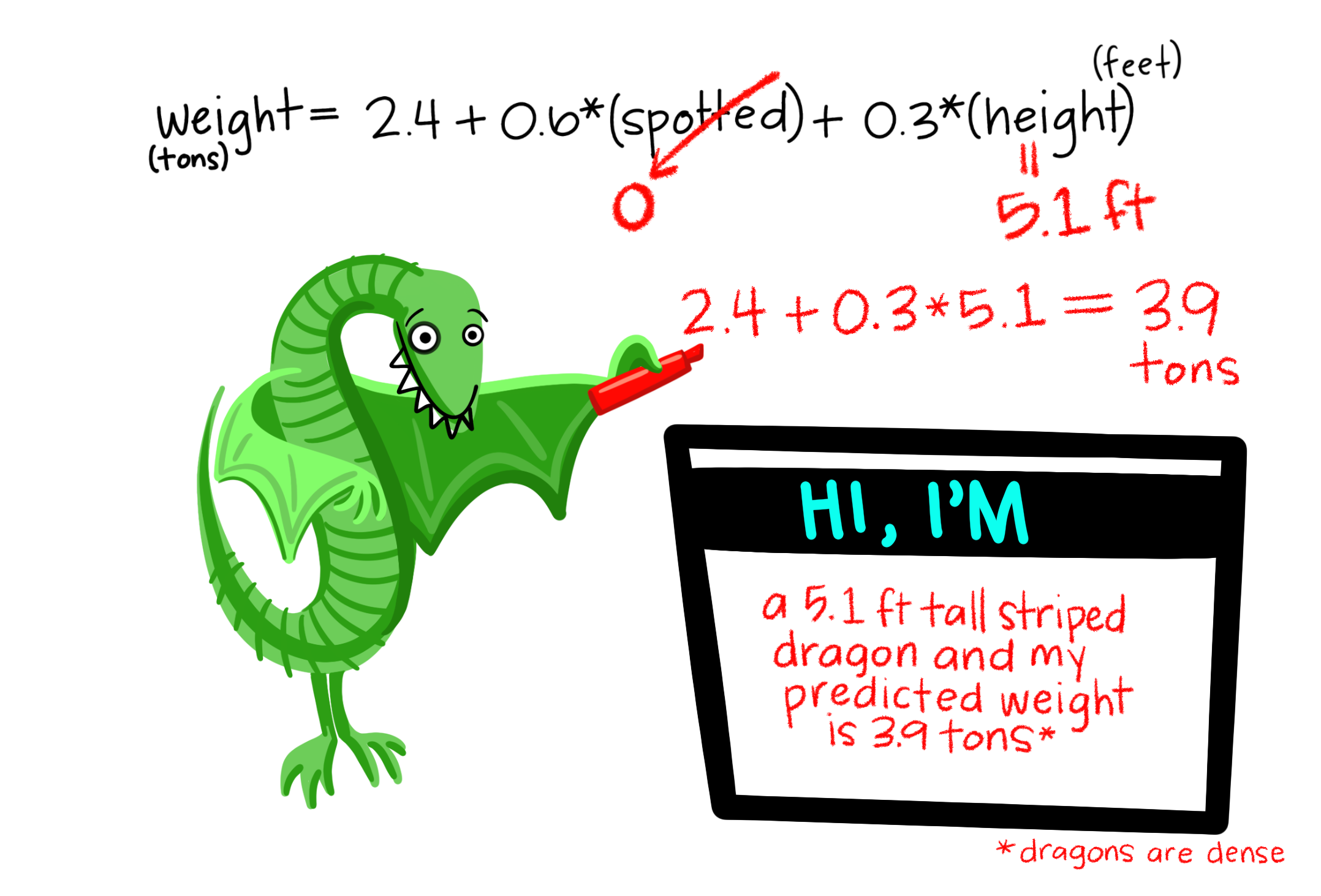
Given response $Y$ and predictors $X_1,\ldots,X_p$, in a linear regression model, we posit:

\[ Y = \beta_0 + \beta_1 X_1 + \ldots + \beta_p X_p + \epsilon, \quad \text{where $\epsilon \sim N(0,\sigma^2)$} \]

Goal is to estimate parameters, also called coefficients $\beta_0,\beta_1,\ldots,\beta_p$

17.3 Sample data

Let’s consider 2 dimensions and instead of calculating univariate statistics by groups (or factors) of other variable - we will measure their common relationships based on co-variance and correlation coefficients and construct a simple linear function of regression.

Our dataset contains information about a random sample of apartments. This data can be used for a lot of purposes such as price prediction to exemplify the use of linear regression in Machine Learning.

The columns in the given dataset is as follows:

price_PLN
price_EUR
rooms
size (sq meters)
district
building_type

17.3.1 Univariate analysis

Recall that we discussed characteristics such as center, spread, and shape. It’s also useful to be able to describe the relationship of two numerical variables, such as price_PLN and size above.

We can also describe the relationship between these two variables using the univariate analysis of the response variable by groups of the independent variable (explanatory). Make sure to discuss the form, direction, and strength of the relationship as well as any unusual observations.

17.3.2 Scatterplots

First let’s visualize our quantitative relationships using scatterplots.

#install.packages("ggplot2", dependencies=TRUE)
library(ggplot2)
# Basic scatter plot
ggplot(apartments, aes(x=size, y=price_PLN)) +
  geom_point(size=2, shape=23)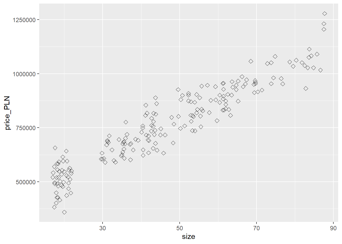

*If the distribution of the response variable is skewed - don’t forget about the necessary transformations (i.e. log function).

17.3.3 Batter up

Our aim is to summarize relationships both graphically and numerically in order to find which variable, if any, helps us best predict the total amount of $ spent in our restaurant.

Broadly speaking, we would like to model the relationship between $X$ and $Y$ using the form

\[ Y = f(X) + \epsilon. \]

The function $f$ describes the functional relationship between the two variables, and the $\epsilon$ term is used to account for error. This indicates that if we plug in a given value of $X$ as input, our output is a value of $Y$, within a certain range of error. You could think of this a number of ways:

Response = Prediction + Error
Response = Signal + Noise
Response = Model + Unexplained
Response = Deterministic + Random
Response = Explainable + Unexplainable

Ok, if the relationship looks linear, we can quantify the strength of the relationship with the Pearson’s correlation coefficient.

cor(apartments$price_PLN, apartments$size)

## [1] 0.9453427

17.4 Sum of squared residuals

Think back to the way that we described the distribution of a single variable.

Just as we used the mean and standard deviation to summarize a single variable, we can summarize the relationship between these two variables by finding the line that best follows their association. Use the following interactive function to select the line that you think does the best job of going through the cloud of points.

#install.packages("statsr")
library(statsr)
plot_ss(x = size, y = price_PLN, data=apartments)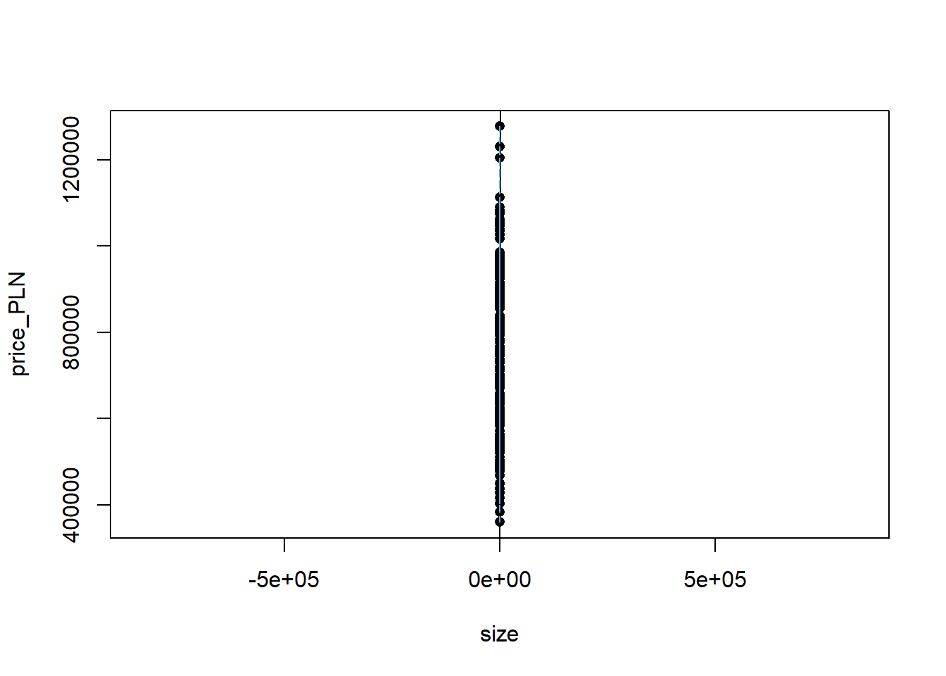

## Click two points to make a line.
                                
## Call:
## lm(formula = y ~ x, data = pts)
## 
## Coefficients:
## (Intercept)            x  
##      355269         8762  
## 
## Sum of Squares:  7.32806e+11

After running this command, you’ll be prompted to click two points on the plotto define a line. Once you’ve done that, the line you specified will be shown in black and the residuals in blue. Note that there are 50 residuals, one for each of the 50 customers. Recall that the residuals are the difference between the observed values and the values predicted by the line:

\[ e_i = y_i - \hat{y}_i \]

The most common way to do linear regression is to select the line that minimizes the sum of squared residuals. To visualize the squared residuals, you can rerun the plot command and add the argument showSquares = TRUE.

plot_ss(x = size, y = price_PLN, data=apartments, showSquares = TRUE)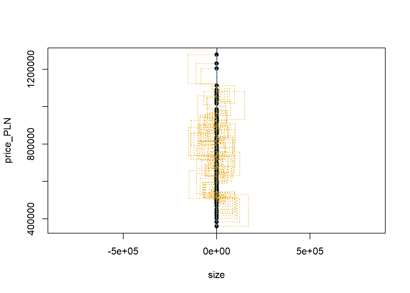

## Click two points to make a line.
                                
## Call:
## lm(formula = y ~ x, data = pts)
## 
## Coefficients:
## (Intercept)            x  
##      355269         8762  
## 
## Sum of Squares:  7.32806e+11

Note that the output from the plot_ss function provides you with the slope and intercept of your line as well as the sum of squares.

Using plot_ss, choose a line that does a good job of minimizing the sum of squares. Run the function several times. What was the smallest sum of squares that you got? How does it compare to your friends (send a message on chat).

17.5 The linear model

It is rather cumbersome to try to get the correct least squares line, i.e. the line that minimizes the sum of squared residuals, through trial and error.

Instead we can use the lm function in R to fit the linear model (a.k.a. regression line).

We can use lm() to fit a linear regression model. The first argument is a formula, of the form Y ~ X1 + X2 + ... + Xp, where Y is the response and X1, …, Xp are the predictors. These refer to column names of variables in a data frame, that we pass in through the data argument.

model1 <- lm(price_PLN ~ size, data = apartments)

The first argument in the function lm is a formula that takes the form y ~ x. Here it can be read that we want to make a linear model of price_PLN as a function of size. The second argument specifies that R should look in the apartments data frame to find the price_PLN and size variables.

The output of lm is an object that contains all of the information we needabout the linear model that was just fit. We can access this information using the summary function.

summary(model1)

## 
## Call:
## lm(formula = price_PLN ~ size, data = apartments)
## 
## Residuals:
##     Min      1Q  Median      3Q     Max 
## -170735  -40337   -5216   40794  154018 
## 
## Coefficients:
##             Estimate Std. Error t value Pr(>|t|)    
## (Intercept) 355269.3    10814.5   32.85   <2e-16 ***
## size          8761.7      214.8   40.79   <2e-16 ***
## ---
## Signif. codes:  0 '***' 0.001 '**' 0.01 '*' 0.05 '.' 0.1 ' ' 1
## 
## Residual standard error: 60840 on 198 degrees of freedom
## Multiple R-squared:  0.8937, Adjusted R-squared:  0.8931 
## F-statistic:  1664 on 1 and 198 DF,  p-value: < 2.2e-16

Let’s consider this output piece by piece. First, the formula used to describe the model is shown at the top. After the formula you find the five-number summary of the residuals. The “Coefficients” table shown next is key; its first column displays the linear model’s y-intercept and the coefficient of log_income. With this table, we can write down the least squares regression line for the linear model:

\[ \hat{y} = 355269.3 + 8761.7 * size \]

One last piece of information we will discuss from the summary output is the Multiple R-squared, or more simply, $R^2$. The $R^2$ value represents the proportion of variability in the response variable that is explained by the explanatory variable. For this model, 89.37% of the variability of apartments in prices (in PLN) is explained by size in square meters.

So… to sum up:

We may then interpret coefficients for categorical predictor variables:

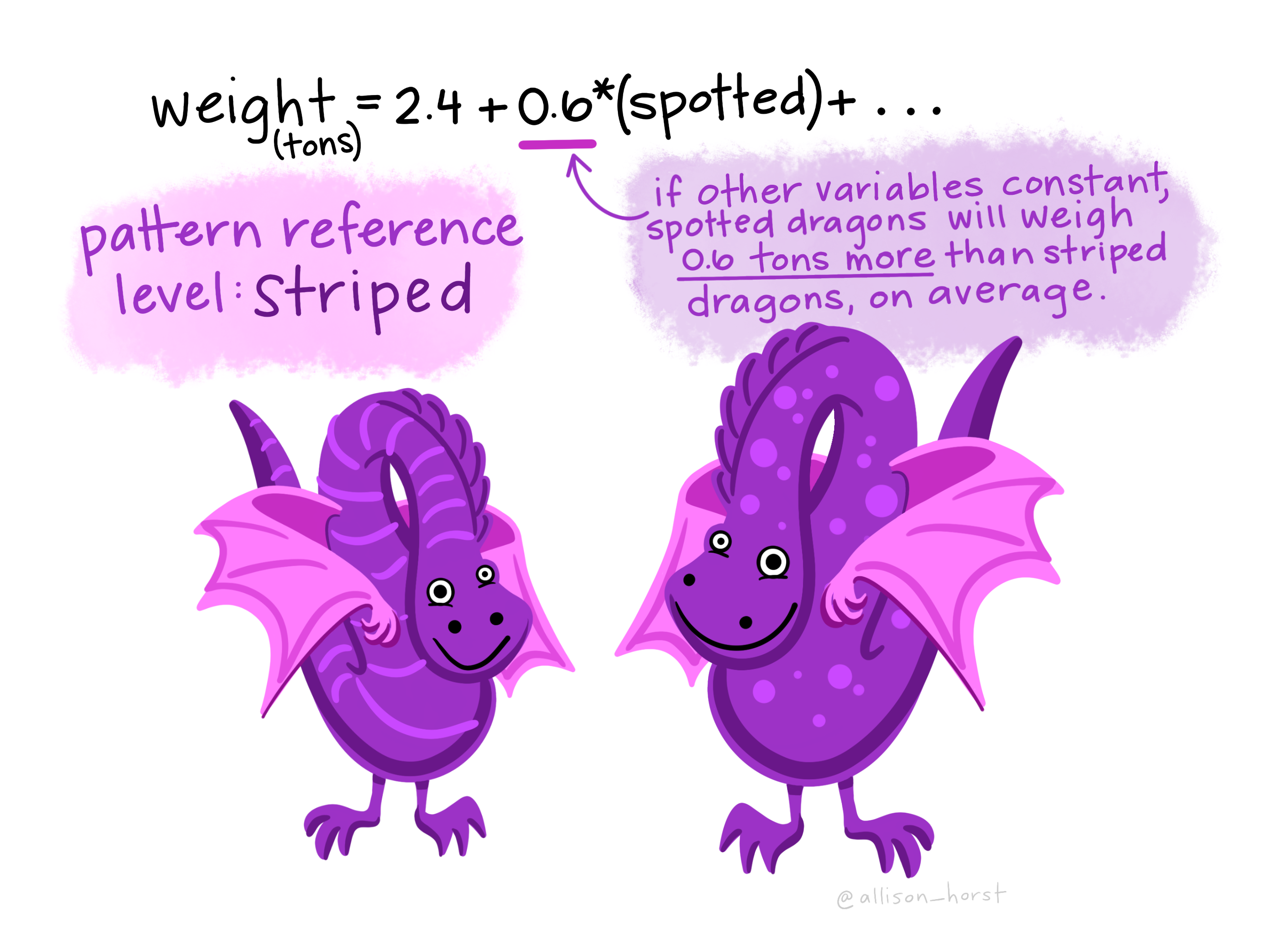
And for continuous predictor variables:

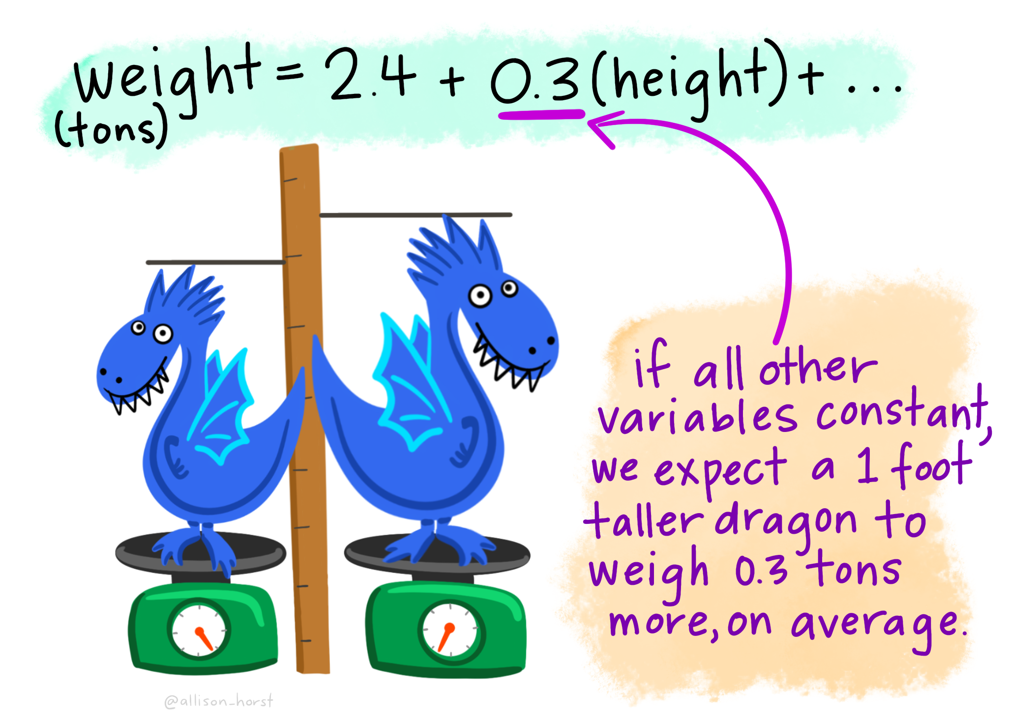
17.6 Prediction and prediction errors

Let’s create a scatterplot with the least squares line laid on top.

attach(apartments)
hist(apartments$price_PLN)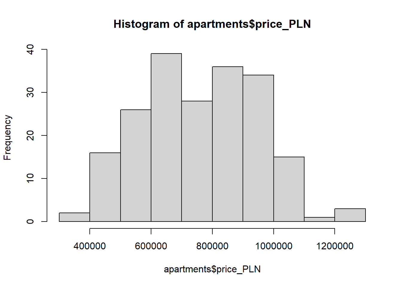

ggplot(apartments, aes(x=size, y=price_PLN)) + 
  geom_point(shape=18, color="blue")+
  geom_smooth(method=lm,  linetype="dashed",
             color="darkred", fill="blue")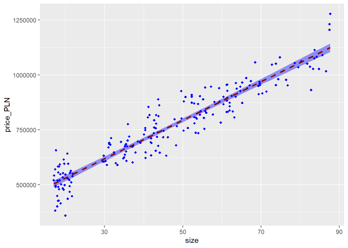

The function abline plots a line based on its slope and intercept. Here, we used a shortcut by providing the model model1, which contains both parameter estimates. This line can be used to predict $y$ at any value of $x$. When predictions are made for values of $x$ that are beyond the range of the observed data, it is referred to as extrapolation and is not usually recommended. However, predictions made within the range of the data are more reliable. 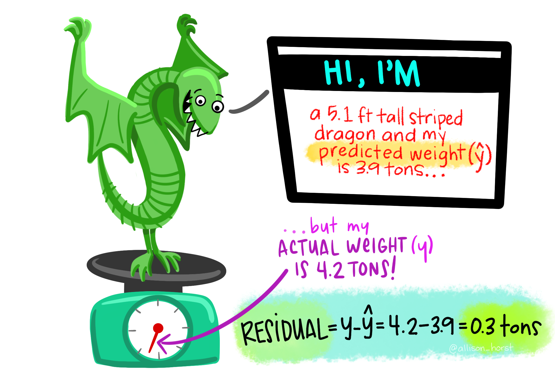They’re also used to compute the residuals.

If a real estate manager saw the least squares regression line and not the actual data, what price (in PLN) would he or she predict for an apartment to have 50 sq. meters? Is this an overestimate or an underestimate, and by how much? In other words, what is the residual for this prediction?

So… we can make predictions using the regression model:

17.7 Model diagnostics

To assess whether the linear model is reliable, we need to check for (1) linearity, (2) nearly normal residuals, and (3) constant variability.

Linearity: We already checked if the relationship between price_PLN and size is linear using a scatterplot. We should also verify this condition with a plot of the residuals vs. size. Recall that any code following a # is intended to be a comment that helps understand the code but is ignored by R.

plot(model1$residuals ~ apartments$size)
abline(h = 0, lty = 3)  # adds a horizontal dashed line at y = 0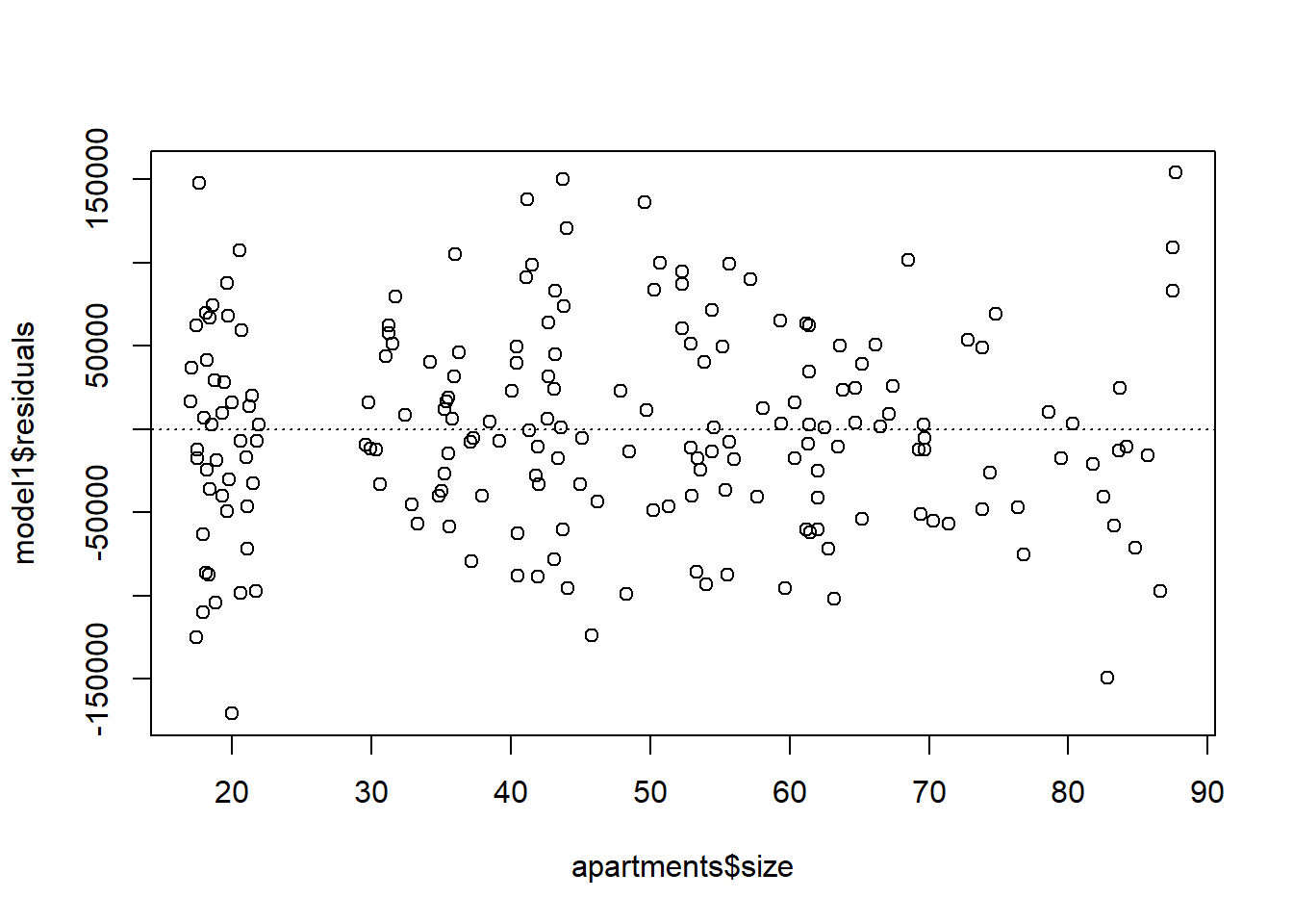

We can also verify linearity using some external libraries.

# Assessing linearity
library(car)
crPlots(model1)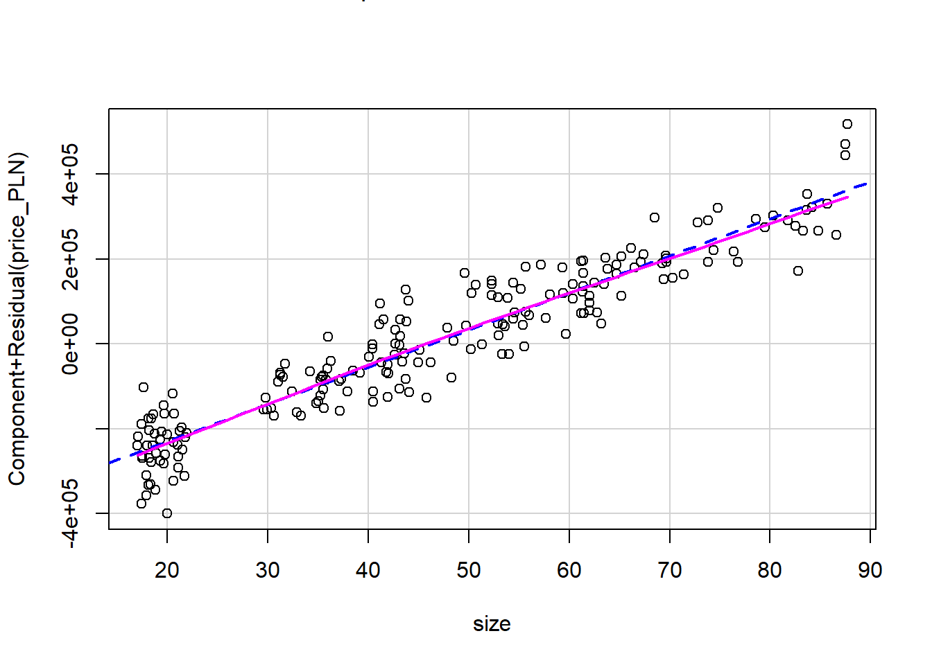

Is there any apparent pattern in the residuals plot? What does this indicate about the linearity of the relationship between runs and at-bats?

Nearly normal residuals: To check this condition, we can look at a histogram of residuals:

hist(model1$residuals)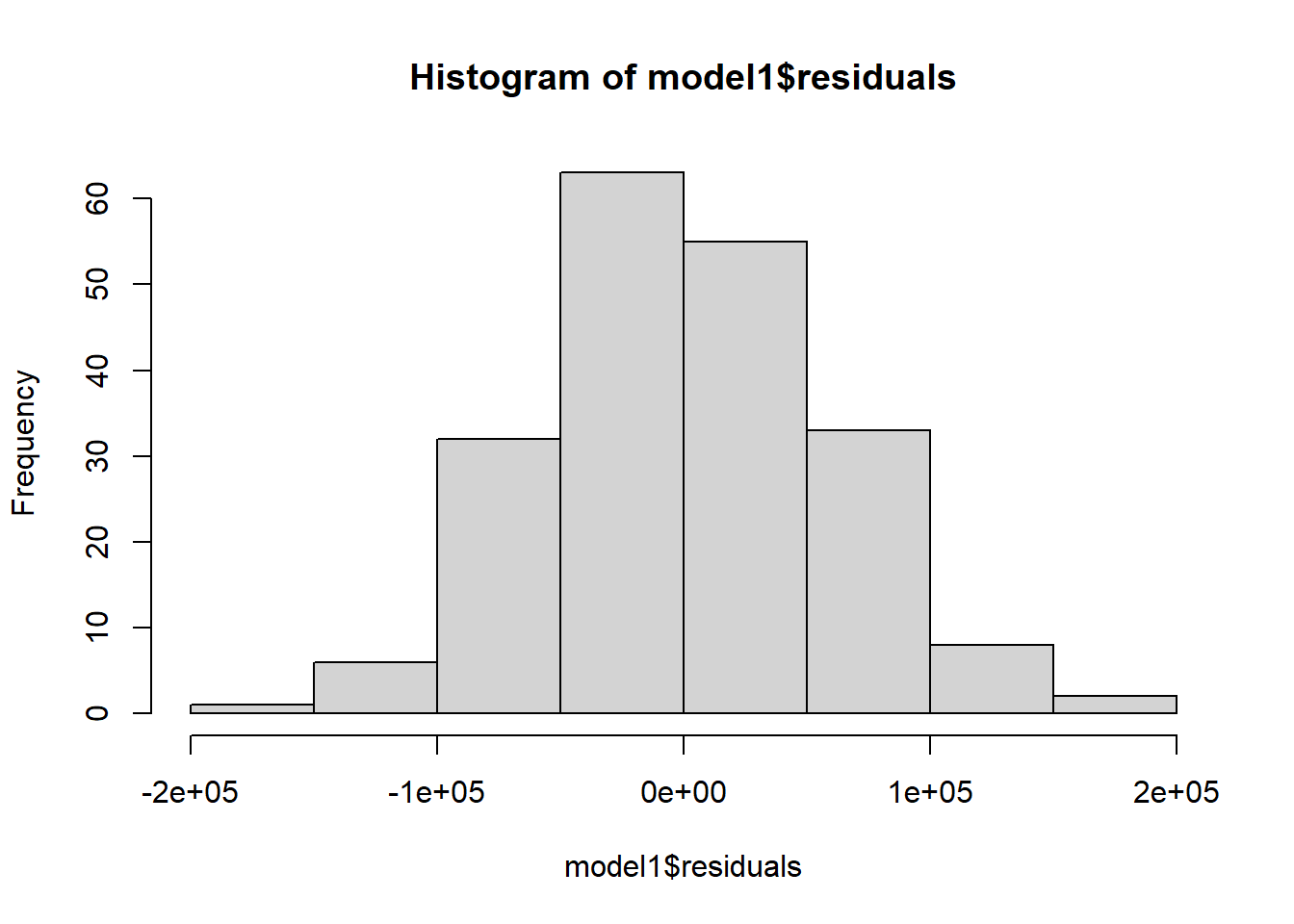

or a normal probability plot of the residuals.

qqnorm(model1$residuals)
qqline(model1$residuals)  # adds diagonal line to the normal prob plot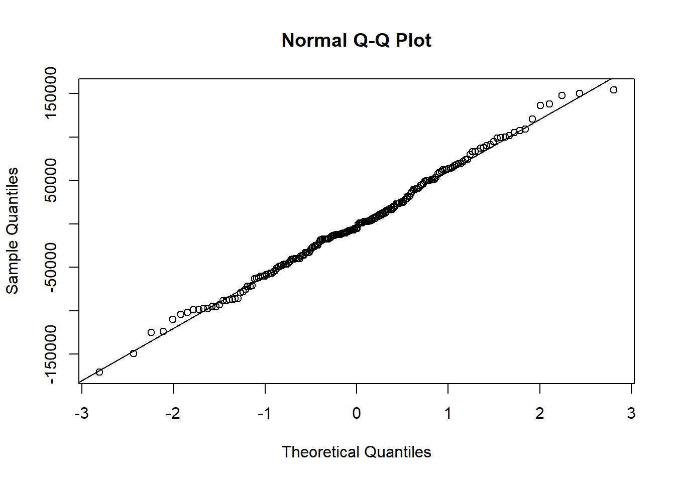

Based on the histogram and the normal probability plot, does the nearly normal residuals condition appear to be met?

Constant variability:

# Assessing homoscedasticity
library(car)
ncvTest(model1)

## Non-constant Variance Score Test 
## Variance formula: ~ fitted.values 
## Chisquare = 0.02459333, Df = 1, p = 0.87538

spreadLevelPlot(model1)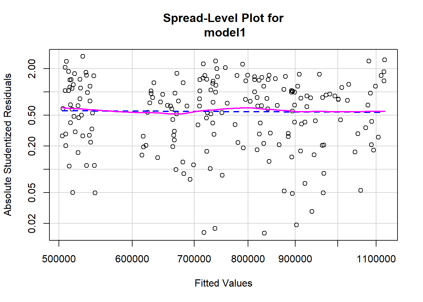

## 
## Suggested power transformation:  1.066677

Based on the plot in (1), does the constant variability condition appear to be met?

# Global test of linear model assumptions
#install.packages("gvlma")
library(gvlma)
gvmodel <- gvlma(model1) 
summary(gvmodel)

## 
## Call:
## lm(formula = price_PLN ~ size, data = apartments)
## 
## Residuals:
##     Min      1Q  Median      3Q     Max 
## -170735  -40337   -5216   40794  154018 
## 
## Coefficients:
##             Estimate Std. Error t value Pr(>|t|)    
## (Intercept) 355269.3    10814.5   32.85   <2e-16 ***
## size          8761.7      214.8   40.79   <2e-16 ***
## ---
## Signif. codes:  0 '***' 0.001 '**' 0.01 '*' 0.05 '.' 0.1 ' ' 1
## 
## Residual standard error: 60840 on 198 degrees of freedom
## Multiple R-squared:  0.8937, Adjusted R-squared:  0.8931 
## F-statistic:  1664 on 1 and 198 DF,  p-value: < 2.2e-16
## 
## 
## ASSESSMENT OF THE LINEAR MODEL ASSUMPTIONS
## USING THE GLOBAL TEST ON 4 DEGREES-OF-FREEDOM:
## Level of Significance =  0.05 
## 
## Call:
##  gvlma(x = model1) 
## 
##                     Value p-value                Decision
## Global Stat        1.9143  0.7515 Assumptions acceptable.
## Skewness           0.3701  0.5429 Assumptions acceptable.
## Kurtosis           0.1054  0.7454 Assumptions acceptable.
## Link Function      1.1400  0.2856 Assumptions acceptable.
## Heteroscedasticity 0.2988  0.5846 Assumptions acceptable.

Now, let’s watch the tutorial on LM diagnostics: