Chapter 4 R-Markdown
Data analysts use R Markdown documents to create repeatable code that can be rendered in a variety of output types. Some of the most popular output types are HTML, Word, and PDF, but new enhancements also allow for PowerPoint presentations.
R Markdown provides an authoring framework for data science. You can use a single R Markdown file to both
- save and execute code
- generate high quality reports that can be shared with an audience
R Markdown documents are fully reproducible and support dozens of static and dynamic output formats. This 1-minute video provides a quick tour of what’s possible with R Markdown:
4.1 Installation
Like the rest of R, R Markdown is free and open source. You can install
the R Markdown package from CRAN with: install.packages("rmarkdown")
4.2 Resources
The links to the left provide a quick tour of R Markdown. The links at the top provide examples of R Markdown documents, as well as an in depth discussion of various R Markdown topics.
You may also find the following resources helpful:
4.3 Introduction
R Markdown is a file format for making dynamic documents with R. An R Markdown document is written in markdown (an easy-to-write plain text format) and contains chunks of embedded R code, like the Figure 4.1 below.
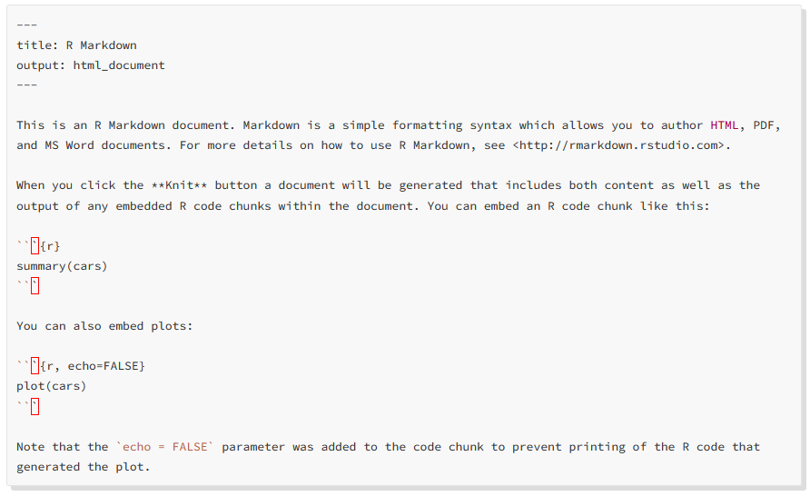
Figure 4.1: R Markdown basic syntax.
R Markdown files are the source code for rich, reproducible documents. You can transform an R Markdown file in two ways.
knit - You can knit the file. The rmarkdown package will call the knitr package. knitr will run each chunk of R code in the document and append the results of the code to the document next to the code chunk. This workflow saves time and facilitates reproducible reports.
Consider how authors typically include graphs (or tables, or numbers) in a report. The author makes the graph, saves it as a file, and then copy and pastes it into the final report. This process relies on manual labor. If the data changes, the author must repeat the entire process to update the graph.
In the R Markdown paradigm, each report contains the code it needs to make its own graphs, tables, numbers, etc. The author can automatically update the report by re-knitting.
convert - You can convert the file. The rmarkdown package will use the pandoc program to transform the file into a new format. For example, you can convert your .Rmd file into an HTML, PDF, or Microsoft Word file. You can even turn the file into an HTML5 or PDF slideshow. rmarkdown will preserve the text, code results, and formatting contained in your original .Rmd file.
Conversion lets you do your original work in markdown, which is very easy to use. You can include R code to knit, and you can share your document in a variety of formats.
You can manually render an R Markdown file with ‘rmarkdown::render()’. This is what the above document looks like when rendered as a HTML file.
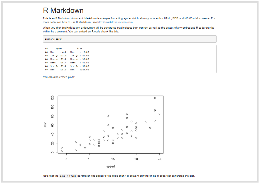
Figure 4.2: R Markdown basic template.
In practice, you do not need to call rmarkdown::render(). You can use a button in the RStudio IDE to render your reprt. R Markdown is heavily integrated into the RStudio IDE.
4.4 R Markdown in RStudio
The RStudio IDE contains many features that make it easy to write and run interactive documents. This article will highlight some of the most useful:
File templates
Using R Markdown
Markdown Quick Reference
The Run Document button
The Viewer Pane Document options
Insert Chunk
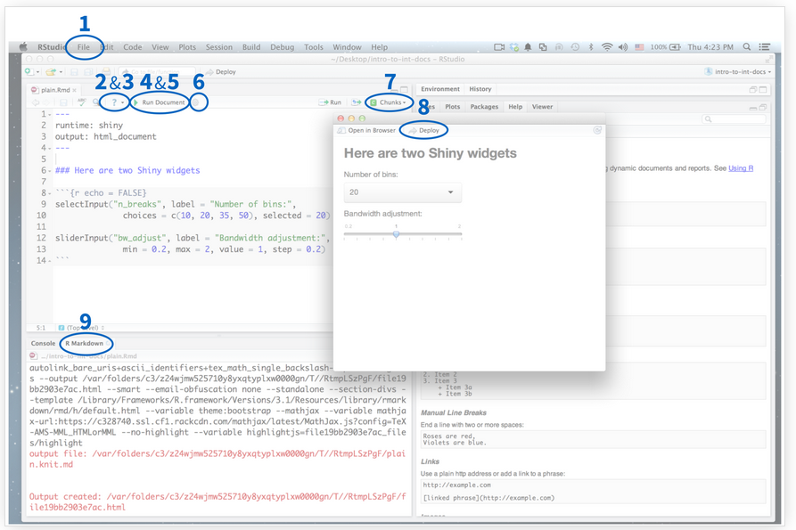
Figure 4.3: R Markdown R Studio IDE.
4.4.0.1 File templates
The RStudio IDE provides a template document when you open a new .Rmd file. To open a new file, click File > New File > R Markdown in the RStudio menu bar.
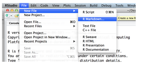
Figure 4.4: R Markdown file design.
A window will pop up that helps you build the YAML frontmatter for the .Rmd file:
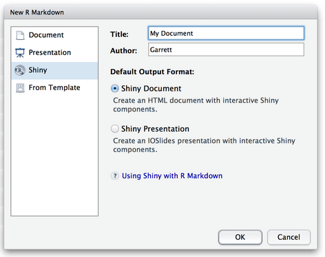
Figure 4.5: R Markdown YAML section design.
From the window’s sidebar, select the category of output that you plan to convert your .Rmd file into. You can select
- Document - a static document
- Presentation - an ioslides or beamer slideshow
- Shiny - an interactive document
- From Template - a format that you have pre-saved as a template (if you have one i.e. *rmdtemplate” package)
Use the radio buttons to select the specific type of output that you wish to build. Your options will depend on the category you selected in the sidebar.
You can also use the window to give your file a title and author field.
To make an interactive document, select Shiny from the sidebar and Shiny Document from the radio buttons. Then click OK.
RStudio will open a new .Rmd file for you to use. The file will contain a YAML header that includes all of the parameters that your file will need to correctly render with ‘rmarkdown::render()’.
RStudio will fill the rest of the file with a template that demonstrates the basic features of .Rmd files. The templates work right out of the box, which means that you can immediately knit or run one.
4.4.0.2 Using R Markdown
The IDE places a question mark icon in the scripts pane whenever you open a .Rmd file. The question mark opens a drop down menu with two helpful resources.
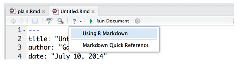
Figure 4.6: R Markdown in R Studio - basic usage.
The first option, “Using R Markdown,” opens the development website for the rmarkdown package, rmarkdown.rstudio.com. Here you can look up the many useful features of R Markdown.
4.4.0.3 Markdown Quick Reference
The second link, “Markdown Quick Reference,” opens a reference guide to the markdown syntax. This guide will appear in the help pane of the RStudio IDE.
The guide uses examples to explain the different formatting options of markdown. It is like a markdown cheat sheet that is built right in to the RStudio IDE.
4.4.0.4 The Run Document button
If your .Rmd file contains runtime: shiny in its YAML header, the RStudio IDE will display a “Run Document” button at the top of the scripts pane.
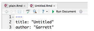
Figure 4.7: R Markdown run button.
The “Run Document” button is a shortcut for the rmarkdown::render command. It let’s you quickly render your .Rmd file into an interactive document hosted locally on your computer. The RStudio IDE will diplay your document in a preview window.
You can edit the .Rmd file while the preview is running. To see your changes, save the .Rmd file. Then click the refresh icon in the top left corner of the preview window.
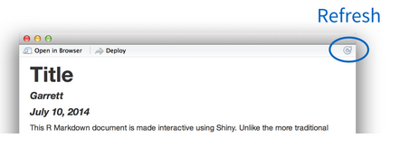
Figure 4.8: R Markdown preview window.
If your .Rmd file does not contain runtime: shiny, the RStudio IDE will display a “Knit HTML” button in place of the “Run Document” button. The “Knit HTML” button works in the same way. It renders your .Rmd file and launches a preview of your output document.
The Knit HTML button contains a dropdown menu that let’s you choose which type of output to knit your file into (this will override the output type specified in your file’s YAML header).
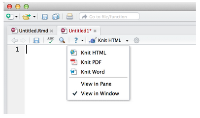
Figure 4.9: R Markdown formatting button.
4.4.0.5 Viewer Pane
By default, the RStudio IDE opens a preview window to display the output of your .Rmd file. However, you can choose to display the output in a dedicated viewer pane.
To do this, select “View in Pane” for m the drop down menu that appears when you click on the “Run Document” button (or “Knit HTML” button).
The viewer pane provides a side-by-side view that resembles some text and Latex editors.
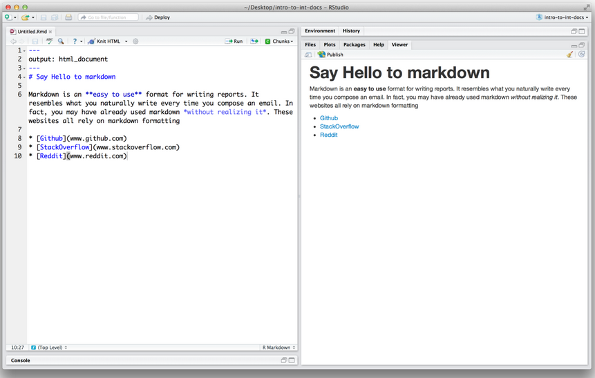
Figure 4.10: R Markdown Viewer Pane.
4.4.0.6 Document options
The gear icon beside “Run Document” opens a wizard that lets you customize your interactive document. You can use this wizard to
- Include a table of contents
- Apply syntax highlighting to code chunks
- Apply one of eight built in bootstrap CSS themes to your document
- Link to your own custom CSS file to style your document
- Number section headings
- Size figures and add captions, and
- Tweak the render process
Set the features you like, and the RStudio IDE will apply them when you click “Run Document”.
4.4.0.7 Insert Chunk
The Chunks button in the top left corner of the Scripts pane opens a dropdown menu that you can use to manage code chunks in your .Rmd file.
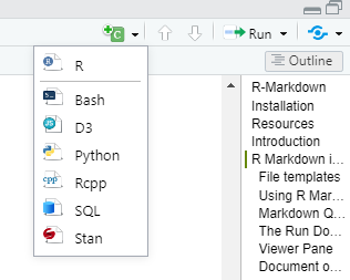
Figure 4.11: R Markdown Insert Chunk button.
The first option in the menu is the most useful. “Insert Chunk” will insert a blank code chunk into your .Rmd file at the location of your cursor. You can then fill this chunk with code.
Code Languages
Notice how this .Rmd file executes code in bash and python. You can open the file here in RStudio Cloud.
knitr can execute code in many languages besides R. Some of the available language engines include:
- Python
- SQL
- Bash
- Rcpp
- Stan
- JavaScript
- CSS
4.5 Getting started
To create an R Markdown report, open a plain text file and save it with the extension .Rmd. You can open a plain text file in your scripts editor by clicking File > New File > Markdown in the RStudio toolbar.
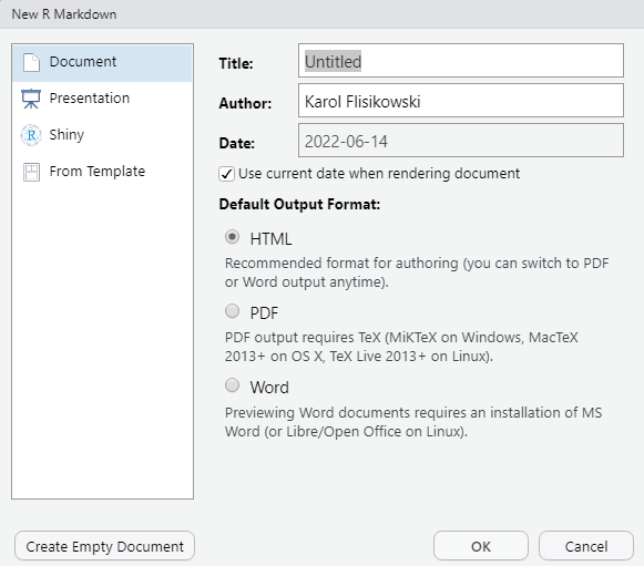
Figure 4.12: R Markdown file in R Studio.
R Markdown reports rely on three frameworks:
- markdown for formatted text
- knitr for embedded R code
- YAML for render parameters
The sections below describe each framework.
4.5.0.1 RMD for text
.Rmd files are meant to contain text written in markdown. Markdown is a set of conventions for formatting plain text. You can use markdown to indicate
- bold and italic text
- lists
- headers (e.g., section titles)
- hyperlinks
- and much more…
The conventions of markdown are very unobtrusive, which make Markdown files easy to read. The Figure 4.13 below. below uses several of the most useful markdown conventions.
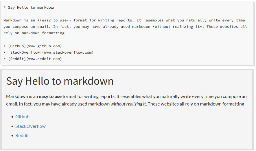
Figure 4.13: R Markdown for text formatting.
The file demonstrates how to use markdown to indicate:
headers - Place one or more hashtags at the start of a line that will be a header (or sub-header). For example, # Say Hello to markdown. A single hashtag creates a first level header. Two hashtags, ##, creates a second level header, and so on.
italicized and bold text - Surround italicized text with asterisks, like this without realizing it. Surround bold text with two asterisks, like this easy to use.
lists - Group lines into bullet points that begin with asterisks. Leave a blank line before the first bullet, like this:
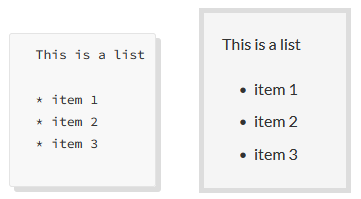
Figure 4.14: R Markdown lists formatting.
- hyperlinks - Surround links with brackets, and then provide the link target in parentheses, like this Github.
You can learn about more of markdown’s conventions in the Markdown Quick Reference guide, which comes with the RStudio IDE.
To access the guide, open a .md or .Rmd file in RStudio. Then click the question mark that appears at the top of the scripts pane. Next, select “Markdown Quick Reference”. RStudio will open the Markdown Quick Reference guide in the Help pane.
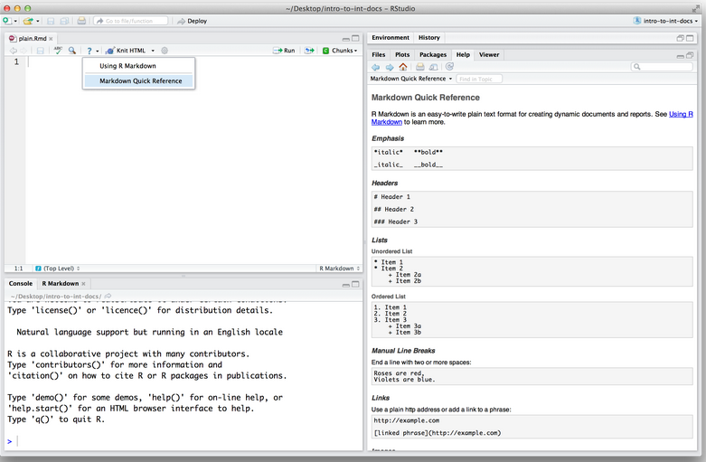
Figure 4.15: R Markdown Quick Reference Guide.
4.5.0.2 Rendering
To transform your markdown file into an HTML, PDF, or Word document, click the “Knit” icon that appears above your file in the scripts editor. A drop down menu will let you select the type of output that you want.
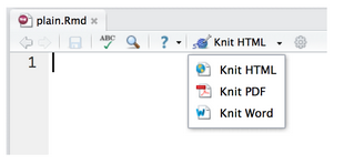
Figure 4.16: R Markdown document rendering.
When you click the button, rmarkdown will duplicate your text in the new file format. rmarkdown will use the formatting instructions that you provided with markdown syntax.
Once the file is rendered, RStudio will show you a preview of the new output and save the output file in your working directory.
Here is how the markdown script above would look in each output format:
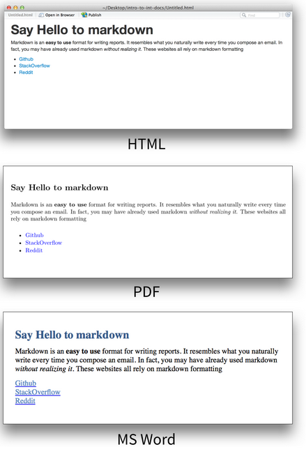
Figure 4.17: R Markdown document rendering to PDF/Word/HTML.
Note: RStudio does not build PDF and Word documents from scratch. You will need to have a distribution of Latex installed on your computer to make PDFs and Microsoft Word (or a similar program) installed to make Word files.
4.5.0.3 Embedded R code
The knitr package extends the basic markdown syntax to include chunks of executable R code.
When you render the report, knitr will run the code and add the results to the output file. You can have the output display just the code, just the results, or both.
To embed a chunk of R code into your report, surround the code with two lines that each contain three backticks. After the first set of backticks, include {r}, which alerts knitr that you have included a chunk of R code. The result will look like this:
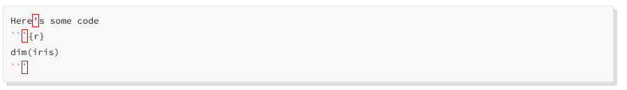
Figure 4.18: R Markdown R code embedding.
When you render your document, knitr will run the code and append the results to the code chunk. knitr will provide formatting and syntax highlighting to both the code and its results (where appropriate).
As a result, the markdown snippet above will look like this when rendered (to HTML).
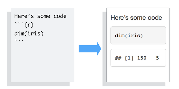
Figure 4.19: R Markdown R code embedded to HTML document.
To omit the results from your final report (and not run the code) add the argument eval = FALSE inside the brackets and after r. This will place a copy of your code into the report.
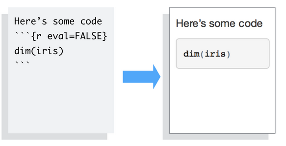
Figure 4.20: R Markdown with omitted results from your final report.
To omit the code from the final report (while including the results) add the argument echo = FALSE. This will place a copy of the results into your report.
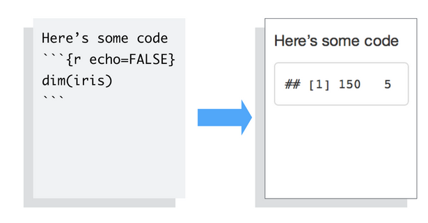
Figure 4.21: R Markdown with omitted code from your final report.
‘echo = FALSE’ is very handy for adding plots to a report, since you usually do not want to see the code that generates the plot.
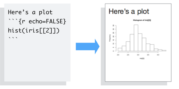
Figure 4.22: R Markdown with omitted code from your final report.
echo and eval are not the only arguments that you can use to customize code chunks. You can learn more about formatting the output of code chunks at the rmarkdown and knitr websites.
4.5.0.4 Inline code
To embed R code in a line of text, surround the code with a pair of backticks and the letter r, like this:

Figure 4.23: R code in a line of a text in HTML document.
knitr will replace the inline code with its result in your final document (inline code is always replaced by its result). The result will appear as if it were part of the original text. For example, the snippet above will appear like this:
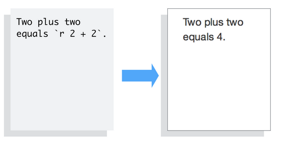
Figure 4.24: Rendered document with R code in a line of a text.
4.5.0.5 YAML for render parameters
You can use a YAML header to control how rmarkdown renders your .Rmd file. A YAML header is a section of key: value pairs surrounded by — marks, like on Figure 4.25 below.
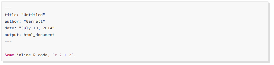
Figure 4.25: Rendered document with R code in a line of a text.
The output: value determines what type of output to convert the file into when you call ‘rmarkdown::render()’. Note: you do not need to specify output: if you render your file with the RStudio IDE knit button.
output: recognizes the following values:
- html_document, which will create HTML output (default)
- pdf_document, which will create PDF output
- word_document, which will create Word output
If you use the RStudio IDE knit button to render your file, the selection you make in the gui will override the output: setting.
4.6 Slideshows
You can also use the output: value to render your document as a slideshow.
- output: ioslides_presentation will create an ioslides (HTML5) slideshow
- output: beamer_presentation will create a beamer (PDF) slideshow
Note: The knit button in the RStudio IDE will update to show slideshow options when you include one of the above output values and save your .Rmd file.
rmarkdown will convert your document into a slideshow by starting a new slide at each header or horizontal rule (e.g., ***).
Visit rmarkdown.rstudio.com to learn about more YAML options that control the render process.
4.7 PowerPoint reports
PowerPoint presentations are still a common format for sharing insights in most organizations today. This tutorial shows you how to create feature-rich PowerPoint presentations from R Markdown and how to use these presentations to share insights, visualizations, Shiny applications, and more.
Please watch this short video-tutorial on how to easily produce PowerPoint presentations with Markdown!