Chapter 3 R-Basics
Technical Notes On R:
When you start a new problem, it’s best to delete all the variables to
ensure you don’t accidentally use old data, just type rm(list=ls()).
Note that you will need to reload your data if you need it. When you
close R, you do not need to save the workspace if it asks. Saving the
workspace just saves the variables you have defined.
3.1 Help
R has an inbuilt help facility similar to the man facility of UNIX. To get more information on any specific named function, for example solve, the command is:
help(solve)
An alternative is:
?solve
For a feature specified by special characters, the argument must be enclosed in double or single quotes, making it a “character string”: This is also necessary for a few words with syntactic meaning including if, for and function.
help("something")
Either form of quote mark may be used to escape the other, as in the string “It’s important”. Our convention is to use double quote marks for preference.
On most R installations help is available in HTML format by running:
help.start()
which will launch a Web browser that allows the help pages to be browsed
with hyperlinks. On UNIX, subsequent help requests are sent to the
HTML-based help system. The ‘Search Engine and Keywords’ link in the
page loaded by help.start() is particularly useful as it is contains a
high-level concept list which searches though available functions. It
can be a great way to get your bearings quickly and to understand the
breadth of what R has to offer. The help.search command (alternatively
??) allows searching for help in various ways. For example:
??solve
Try ?help.search for details and more examples.
The examples on a help topic can normally be run by:
example(topic)
Windows versions of R have other optional help systems: use ?help for
further details.
3.2 Data structures
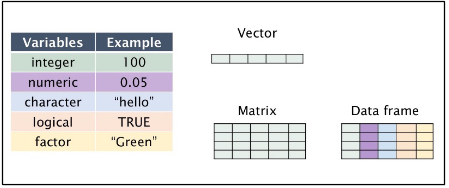
We have several data structures in R:
numeric - numeric data (approximations of the real numbers)
integer - integer data (whole numbers)
factor - categorical data (simple classifications, like gender)
ordered - ordinal data (ordered classifications, like educational level)
character - character data (strings)
raw - binary data
Special observations:
- NA
- NULL
- Inf
- NaN
Conversion of data structures’ types:
- as.numeric
- as.logical
- as.integer
- as.factor
- as.character
- as.ordered
Variables can be thought of as a labelled container used to store information. Variables allow us to recall saved information to later use in calculations. Variables can store many different things in R studio, from single values to tables of information, images and graphs.
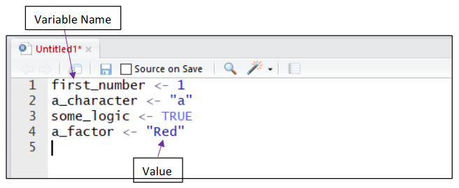
Assigning a Value to a Variable:
Storing a value or “assigning” it to a variable is completed using either <- or = function. The name given to a variable should describe the information or data being stored. This helps when revisiting old code or when sharing it with others.
3.2.1 Vectors
R operates on named data structures. The simplest such structure is the numeric vector, which is a single entity consisting of an ordered collection of numbers. To set up a vector named x, say, consisting of five numbers, namely 10.4, 5.6, 3.1, 6.4 and 21.7, use the R command:
x <- c(10.4, 5.6, 3.1, 6.4, 21.7)
This is an assignment statement using the function c() which in this
context can take an arbitrary number of vector arguments and whose value
is a vector got by concatenating its arguments end to end. A number
occurring by itself in an expression is taken as a vector of length one.
Notice that the assignment operator (<-), which consists of the two
characters < (“less than”) and - (“minus”) occurring strictly
side-by-side and it ‘points’ to the object receiving the value of the
expression. In most contexts the = operator can be used as an
alternative.
Assignment can also be made using the function assign(). An equivalent
way of making the same assignment as above is with:
assign("x", c(10.4, 5.6, 3.1, 6.4, 21.7))
The usual operator, <-, can be thought of as a syntactic short-cut to
this.
3.2.2 Sequences
R has a number of facilities for generating commonly used sequences of
numbers. For example 1:30 is the vector c(1, 2, ..., 29, 30). The colon operator has high priority within an expression, so, for example 2*1:15 is the vector c(2, 4, ..., 28, 30). Put n <- 10 and compare the sequences 1:n-1 and 1:(n-1).
The construction 30:1 may be used to generate a sequence backwards. The function seq() is a more general facility for generating sequences. It has five arguments, only some of which may be specified in any one call. The first two arguments, if given, specify the beginning and end of the sequence, and if these are the only two arguments given the result is the same as the colon operator. That is seq(2,10) is the same vector as 2:10.
Parameters to seq(), and to many other R functions, can also be given in named form, in which case the order in which they appear is irrelevant. The first two parameters may be named from=value and to=value; thus seq(1,30), seq(from=1, to=30) and seq(to=30,from=1) are all the same as 1:30. The next two parameters to seq() may be named by=value and length=value , which specify a step size and a length for the sequence respectively. If neither of these is given, the default by=1 is assumed.
For example:
seq(-5, 5, by=.2) -> s3 generates in s3 the vector c(-5.0, -4.8, -4.6,..., 4.6, 4.8, 5.0). Similarly s4 <- seq(length=51, from=-5, by=.2) generates the same vector in s4.
A related function is rep() which can be used for replicating an object in various complicated ways. The simplest form is: s5 <- rep(x, times=5) which will put five copies of x end-to-end in s5.
Another useful version is s6 <- rep(x, each=5) which repeats each element of x five times before moving on to the next.
3.2.3 Factors
A factor is a vector object used to specify a discrete classification (grouping) of the components of other vectors of the same length. R provides both ordered and unordered factors.
Levels of a variable are stored as numbers, labeled as an array of “levels”, but storing a large number of categories as a factor takes up a lot of space!
Try:
f <- factor(c("a", "b", "a", "a", "c"))
levels(f)
Recoding:
gender <- c(2, 1, 1, 2, 0, 1, 1)
recode <- c(male = 1, female = 2)
gender <- factor(gender, levels = recode, labels = names(recode))
levels(gender)
gender - and we have 1 NA!
Exercise:
Create a factor named “risk”: third column in “person” frame - for age
<20 years “0” with label “risk”, for age >30 years “1” with label
“none”.
Solution:
person$risk<- as.factor(ifelse(person$age > 30, c("risk"), c("none")))
3.2.4 Data frames
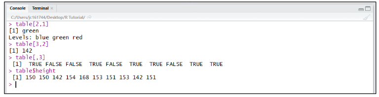
A dataset will often contain more than 1 variable of interest. To combine vectors of the same length together into a table or “dataframe” (similar to an excel table), we use the data.frame() command. Below we have combined 3 vectors (colour, height and survey), containing 10 values each, together into a dataframe. The table has been assigned to the variable table.
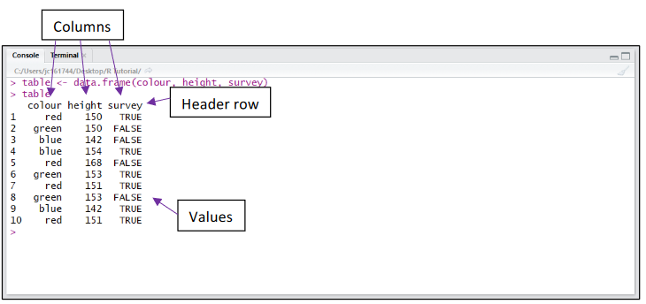
The top line of the dataframe is called the header row and contains a descriptive name for the values in each column.
Below the header row, values can be referred to individually or in whole rows and columns.
To retrieve a single value from a dataframe assigned to a variable, the variable name is used then followed by the coordinates of the value within [row, column] square brackets (eg. table[2,1] returns green and table[3,2] returns 142). Whole rows can be returned individually using coordinates (eg. table[3,] returns all values for row 3). Single columns can be returned by either referring to them using a coordinate with the row blank (eg. table[,3] returns all values in 3rd column), or by using the variable name followed by a $ and the column header (eg. table$height returns all “height” values from the dataframe “table”).
Note: You can find out what type of data is stored within a variable or a column in a dataframe using the class() function.
3.2.5 Tibbles
A tibble, or tbl_df, is a modern reimagining of the data.frame, keeping what time has proven to be effective, and throwing out what is not. Tibbles are data.frames that are lazy and surly: they do less (i.e. they don’t change variable names or types, and don’t do partial matching) and complain more (e.g. when a variable does not exist). This forces you to confront problems earlier, typically leading to cleaner, more expressive code. Tibbles also have an enhanced print() method which makes them easier to use with large datasets containing complex objects.
If you are new to tibbles, the best place to start is the tibbles chapter in R for data science.
3.2.6 Matrix
Matrix is a two dimensional data structure in R programming.
Matrix is similar to vector but additionally contains the dimension attribute. All attributes of an object can be checked with the attributes() function (dimension can be checked directly with the dim() function).
Matrix can be created using the matrix() function.
Dimension of the matrix can be defined by passing appropriate value for arguments nrow and ncol.
Providing value for both dimension is not necessary. If one of the dimension is provided, the other is inferred from length of the data.
> matrix(1:9, nrow = 3, ncol = 3) [,1] [,2] [,3] [1,] 1 4 7 [2,] 2 5 8 [3,] 3 6 9
Same result is obtained by providing only one dimension:
> matrix(1:9, nrow = 3) [,1] [,2] [,3] [1,] 1 4 7 [2,] 2 5 8 [3,] 3 6 9
We can see that the matrix is filled column-wise. This can be reversed to row-wise filling by passing TRUE to the argument byrow.
> matrix(1:9, nrow=3, byrow=TRUE) [,1] [,2] [,3] [1,] 1 2 3 [2,] 4 5 6 [3,] 7 8 9
In all cases, however, a matrix is stored in column-major order internally as we will see in the subsequent sections.
It is possible to name the rows and columns of matrix during creation by passing a 2 element list to the argument dimnames:
x <- matrix(1:9, nrow = 3, dimnames = list(c("X","Y","Z"), c("A","B","C")))
> x A B C X 1 4 7 Y 2 5 8 Z 3 6 9
These names can be accessed or changed with two helpful functions colnames() and rownames().
> colnames(x)
[1] “A” “B” “C”
> rownames(x)
[1] “X” “Y” “Z”
It is also possible to change names:
colnames(x) <- c("C1","C2","C3")
rownames(x) <- c("R1","R2","R3")
x
C1 C2 C3 R1 1 4 7 R2 2 5 8 R3 3 6 9
We can access elements of a matrix using the square bracket [ indexing method. Elements can be accessed as var[row, column]. Here rows and columns are vectors.
Select rows 1 & 2 and columns 2 & 3:
x[c(1,2),c(2,3)]
We can combine assignment operator with the above learned methods for accessing elements of a matrix to modify it.
Modify a single element:
x[2,2] <- 10
3.2.7 List
A list is a generic vector containing other objects.
For example, the following variable x is a list containing copies of three vectors n, s, b, and a numeric value 3.
X contains copies of n, s, b:
n = c(2, 3, 5)
s = c("aa", "bb", "cc", "dd", "ee")
b = c(TRUE, FALSE, TRUE, FALSE, FALSE)
x = list(n, s, b, 3)
3.2.8 Array
Arrays are the R data objects which can store data in more than two dimensions. For example − If we create an array of dimension (2, 3, 4) then it creates 4 rectangular matrices each with 2 rows and 3 columns. Arrays can store only data type.
An array is created using the array() function. It takes vectors as input and uses the values in the dim parameter to create an array.
Example: let’s create an array of two 3x3 matrices each with 3 rows and 3 columns:
Create two vectors of different lengths:
vector1 <- c(5,9,3)vector2 <- c(10,11,12,13,14,15)Take these vectors as input to the array:
result <- array(c(vector1,vector2),dim = c(3,3,2))print(result)
When we execute the above code, it produces the following result:
, , Matrix1
COL1 COL2 COL3ROW1 5 10 13 ROW2 9 11 14 ROW3 3 12 15
, , Matrix2
COL1 COL2 COL3ROW1 5 10 13 ROW2 9 11 14 ROW3 3 12 15
How to access arrays’ elements?
Example: print the element in the 1st row and 3rd column of the 1st matrix:
print(result[1,3,1])
3.3 Dates
Dates are represented as the number of days since 1970-01-01, with negative values for earlier dates.
Use as.Date() to convert strings to dates:
mydates <- as.Date(c("2007-06-22", "2004-02-13"))
Number of days between 6/22/07 and 2/13/04:
days <- mydates[1] - mydates[2]
Sys.Date() returns today’s date. date() returns the current date
and time.
The following symbols can be used with the format() function to print
dates.
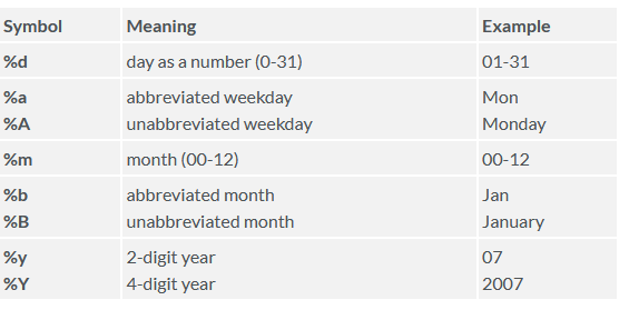
Here is an example: print today’s date:
today <- Sys.Date()
format(today, format="%B %d %Y")
3.3.1 Date Conversion
Character to Date:
You can use the as.Date() function to convert character data to
dates. The format is as.Date(x, "format"), where x is the character
data and format gives the appropriate format.
Example: convert date info in format mm/dd/yyyy:
strDates <- c("01/05/1965", "08/16/1975")
dates <- as.Date(strDates, "%m/%d/%Y")
The default format is yyyy-mm-dd:
mydates <- as.Date(c("2007-06-22", "2004-02-13"))
3.5 Base pipes
As of June 10, the R 4.1 release features a pipe operator that allows so-called “forward” or forward operations, greatly simplifying data analysis and commands. Operations of this type simply mean passing the output argument of one function as the input of the next, and so on, until the final one - usually analytical or graphical.
We write a pipe as: |>
Another, quite commonly used pipe is %>% available in the dplyr and tidyverse packages.
Shortcut: CTRL + SHIFT + M
Example. Draw a density plot from the previously loaded housing price data (the “data” frame):
data <- read.csv(file=“https://tiny.pl/9rs5c”)`
attach(data)
price |> density() |> plot()
As we can see, without specifying plot parameters, variables, operations were performed. There was no need to add objects in memory permanently. Everything was done “on the fly”.
3.6 Tidy pipes
Pipe operators, available in magrittr, dplyr, and other R packages, process a data-object using a sequence of operations by passing the result of one step as input for the next step using infix-operators rather than the more typical R method of nested function calls.
Note that the intended aim of pipe operators is to increase human readability of written code.
The pipe operator is defined in the magrittr package, but it gained huge visibility and popularity with the dplyr package (which imports the definition from magrittr). Now it is part of tidyverse, which is a collection of packages that “work in harmony because they share common data representations and API design”.
The magrittr package also provides several variations of the pipe operator for those who want more flexibility in piping, such as the compound assignment pipe %<>%, the exposition pipe %$%, and the tee operator %T>%. It also provides a suite of alias functions to replace common functions that have special syntax (+, [, [[, etc.) so that they can be easily used within a chain of pipes.
The pipe operator, %>%, is used to insert an argument into a function. It is not a base feature of the language and can only be used after attaching a package that provides it, such as magrittr.
The pipe operator takes the left-hand side (LHS) of the pipe and uses it as the first argument of the function on the right-hand side (RHS) of the pipe.
For example:
library(magrittr)##
## Dołączanie pakietu: 'magrittr'## Następujący obiekt został zakryty z 'package:purrr':
##
## set_names## Następujący obiekt został zakryty z 'package:tidyr':
##
## extract1:10 %>% mean## [1] 5.5is equivalent to:
mean(1:10)## [1] 5.5The pipe can be used to replace a sequence of function calls. Multiple pipes allow us to read and write the sequence from left to right, rather than from inside to out.
The magrittr package contains a compound assignment infix-operator, %<>%, that updates a value by first piping it into one or more rhs expressions and then assigning the result. This eliminates the need to type an object name twice (once on each side of the assignment operator <-). %<>% must be the first infix-operator in a chain:
library(magrittr)
library(dplyr)
df <- mtcars
Instead of writing:
df <- df %>% select(1:3) %>% filter(mpg > 20, cyl == 6)or:
df %>% select(1:3) %>% filter(mpg > 20, cyl == 6) -> dfThe compound assignment operator will both pipe and reassign df:
df %<>% select(1:3) %>% filter(mpg > 20, cyl == 6)