Chapter 18 Multiple Regression
“All models are wrong, but some are useful.”
— George E. P. Box
After reading this chapter you will be able to fit and interpret linear, non-linear multiple regression models, evaluate model assumptions & select the best one among competing models.
18.1 Sample data
Our aim is to predict house values. Before we begin to do any analysis, we should always check whether the dataset has missing value or not, we do so by typing:
houses <- read.csv("real_estates.csv",row.names=1)
attach(houses)
any(is.na(houses))
## [1] FALSELet’s take a look at structure of the data set:
glimpse(houses)## Rows: 506
## Columns: 14
## $ crim <dbl> 0.00632, 0.02731, 0.02729, 0.03237, 0.06905, 0.02985, 0.08829,…
## $ zn <dbl> 18.0, 0.0, 0.0, 0.0, 0.0, 0.0, 12.5, 12.5, 12.5, 12.5, 12.5, 1…
## $ indus <dbl> 2.31, 7.07, 7.07, 2.18, 2.18, 2.18, 7.87, 7.87, 7.87, 7.87, 7.…
## $ chas <int> 0, 0, 0, 0, 0, 0, 0, 0, 0, 0, 0, 0, 0, 0, 0, 0, 0, 0, 0, 0, 0,…
## $ nox <dbl> 0.538, 0.469, 0.469, 0.458, 0.458, 0.458, 0.524, 0.524, 0.524,…
## $ rm <dbl> 6.575, 6.421, 7.185, 6.998, 7.147, 6.430, 6.012, 6.172, 5.631,…
## $ age <dbl> 65.2, 78.9, 61.1, 45.8, 54.2, 58.7, 66.6, 96.1, 100.0, 85.9, 9…
## $ dis <dbl> 4.0900, 4.9671, 4.9671, 6.0622, 6.0622, 6.0622, 5.5605, 5.9505…
## $ rad <int> 1, 2, 2, 3, 3, 3, 5, 5, 5, 5, 5, 5, 5, 4, 4, 4, 4, 4, 4, 4, 4,…
## $ tax <int> 296, 242, 242, 222, 222, 222, 311, 311, 311, 311, 311, 311, 31…
## $ ptratio <dbl> 15.3, 17.8, 17.8, 18.7, 18.7, 18.7, 15.2, 15.2, 15.2, 15.2, 15…
## $ black <dbl> 396.90, 396.90, 392.83, 394.63, 396.90, 394.12, 395.60, 396.90…
## $ lstat <dbl> 4.98, 9.14, 4.03, 2.94, 5.33, 5.21, 12.43, 19.15, 29.93, 17.10…
## $ medv <dbl> 24.0, 21.6, 34.7, 33.4, 36.2, 28.7, 22.9, 27.1, 16.5, 18.9, 15…We should also check if there are any missing or duplicated values:
sum(is.na(houses))## [1] 0sum(duplicated(houses))## [1] 0Our dataset contains information about a random sample of real estates and various characteristics for their neighbourhood.
This data frame has 506 rows and 14 columns (predictors).
We have descriptions and summaries of predictors as follow:
crim: per capita crime rate by town
zn: proportion of residential land zoned for lots over 25,000 sq.ft.
indus: proportion of non-retail business acres per town
chas: river dummy variable (= 1 if tract bounds river; 0 otherwise)
nox: nitrogen oxides concentration (parts per 10 million)
rm: average number of rooms per dwelling
age: proportion of owner-occupied units built prior to 1940
dis: weighted mean of distances to the city employment centres
rad: index of accessibility to radial highways
tax: full-value property-tax rate per $10,000
ptratio: pupil-teacher ratio by town
black: 1000(Bk - 0.63)^2 where Bk is the proportion of blacks by town
lstat: lower status of the population (percent)
medv: median value of owner-occupied homes in $1000s [our dependent variable]
18.1.1 Univariate analysis and correlation plots
- Recall that we discussed characteristics such as center, spread, and shape. We can also describe the relationship between these two variables using the univariate analysis of the response variable “medv” by groups of the independent variable (explanatory).
summary(houses)## crim zn indus chas
## Min. : 0.00632 Min. : 0.00 Min. : 0.46 Min. :0.00000
## 1st Qu.: 0.08205 1st Qu.: 0.00 1st Qu.: 5.19 1st Qu.:0.00000
## Median : 0.25651 Median : 0.00 Median : 9.69 Median :0.00000
## Mean : 3.61352 Mean : 11.36 Mean :11.14 Mean :0.06917
## 3rd Qu.: 3.67708 3rd Qu.: 12.50 3rd Qu.:18.10 3rd Qu.:0.00000
## Max. :88.97620 Max. :100.00 Max. :27.74 Max. :1.00000
## nox rm age dis
## Min. :0.3850 Min. :3.561 Min. : 2.90 Min. : 1.130
## 1st Qu.:0.4490 1st Qu.:5.886 1st Qu.: 45.02 1st Qu.: 2.100
## Median :0.5380 Median :6.208 Median : 77.50 Median : 3.207
## Mean :0.5547 Mean :6.285 Mean : 68.57 Mean : 3.795
## 3rd Qu.:0.6240 3rd Qu.:6.623 3rd Qu.: 94.08 3rd Qu.: 5.188
## Max. :0.8710 Max. :8.780 Max. :100.00 Max. :12.127
## rad tax ptratio black
## Min. : 1.000 Min. :187.0 Min. :12.60 Min. : 0.32
## 1st Qu.: 4.000 1st Qu.:279.0 1st Qu.:17.40 1st Qu.:375.38
## Median : 5.000 Median :330.0 Median :19.05 Median :391.44
## Mean : 9.549 Mean :408.2 Mean :18.46 Mean :356.67
## 3rd Qu.:24.000 3rd Qu.:666.0 3rd Qu.:20.20 3rd Qu.:396.23
## Max. :24.000 Max. :711.0 Max. :22.00 Max. :396.90
## lstat medv
## Min. : 1.73 Min. : 5.00
## 1st Qu.: 6.95 1st Qu.:17.02
## Median :11.36 Median :21.20
## Mean :12.65 Mean :22.53
## 3rd Qu.:16.95 3rd Qu.:25.00
## Max. :37.97 Max. :50.00- It’s also useful to be able to describe the relationship of two variables. Please use the appropriate measures and plots to find significant relationships between our response variable “medv” and the rest of characteristics. Make sure to discuss the form, direction, and strength of the relationship as well as any unusual observations.
#install.packages("corrplot")
library(corrplot)
#checking correlation between variables
corrplot(cor(houses), method = "number", type = "upper", diag =FALSE)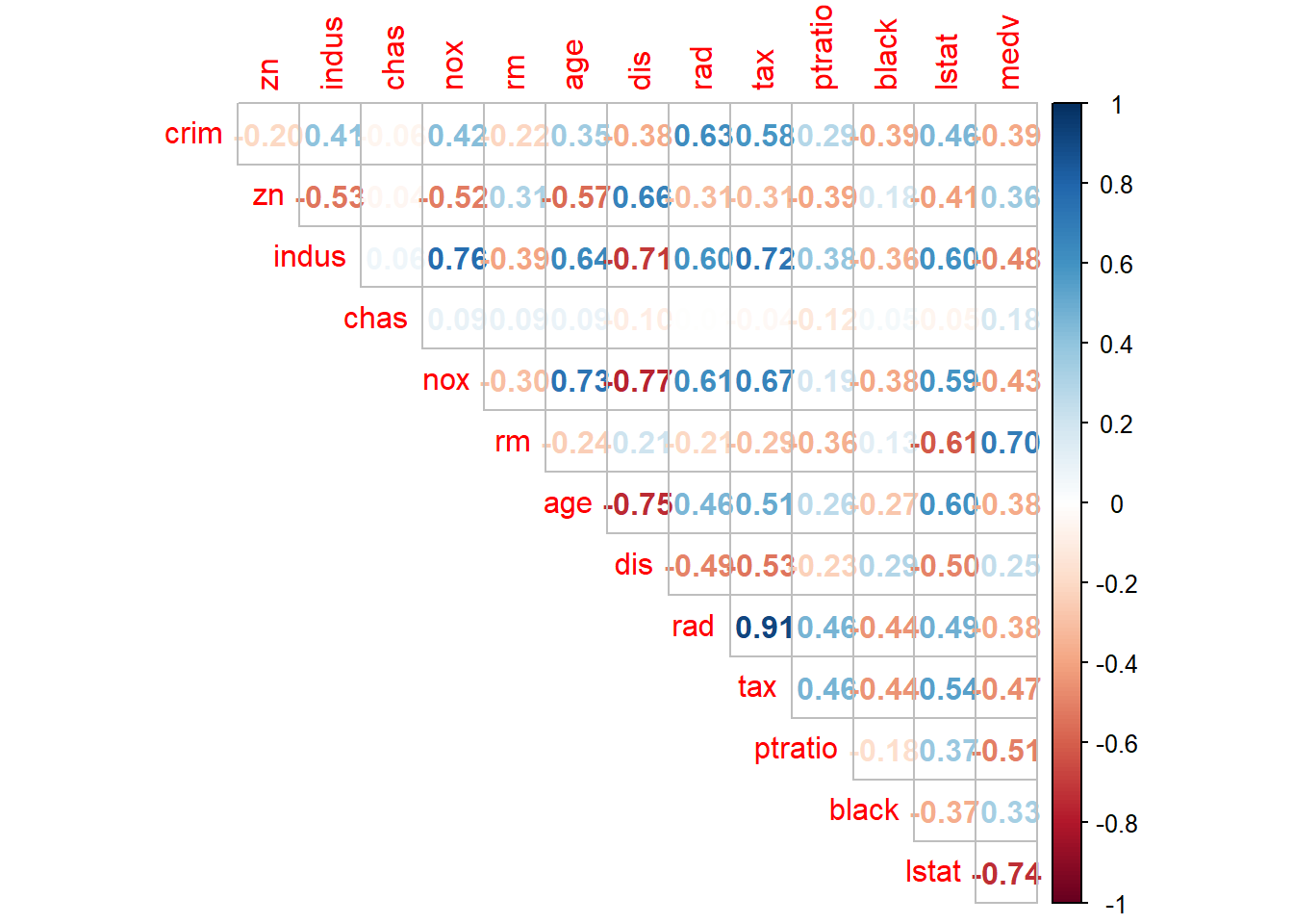
#corr_matrix<-cor(houses)
#corrplot(corr_matrix, type="upper")
There are no missing or duplicate values.
From correlation matrix, some of the observations made are as follows:
- Median value of owner-occupied homes (in 1000$) increases as average number of rooms per dwelling increases and it decreases if percent of lower status population in the area increases
- nox or nitrogen oxides concentration (ppm) increases with increase in proportion of non-retail business acres per town and proportion of owner-occupied units built prior to 1940.
- rad and tax have a strong positive correlation of 0.91 which implies that as accessibility of radial highways increases, the full value property-tax rate per $10,000 also increases.
- crim is strongly associated with variables rad and tax which implies as accessibility to radial highways increases, per capita crime rate increases.
- indus has strong positive correlation with nox, which supports the notion that nitrogen oxides concentration is high in industrial areas.
18.1.2 Scatterplots
First let’s visualize our quantitative relationships using scatterplots.
plot(medv ~ lstat, data = houses,
     xlab = "Lower status of the population (%)",
     ylab = "House value in kUSD",
     main = "House value vs Lower status of the population",
     pch  = 20,
     cex  = 2,
     col  = "grey")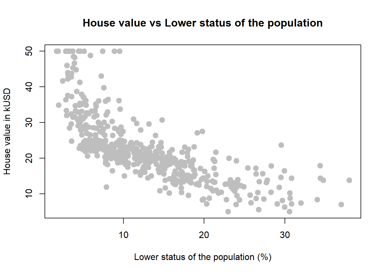
*If the distribution of the response variable is skewed - don’t forget about the necessary transformations (i.e. log function).
18.2 Simple Model
It is rather cumbersome to try to get the correct least squares line, i.e. the line that minimizes the sum of squared residuals, through trial and error.
Instead we can use the lm function in R to fit the linear model (a.k.a. regression line).
We begin by splitting the dataset into two parts, training set and testing set. In this example we will randomly take 75% row in this dataset and put it into the training set, and other 25% row in the testing set:
smp_size<-floor(0.75*nrow(houses))
set.seed(12)
train_ind<-sample(seq_len(nrow(houses)), size=smp_size)
train<-houses[train_ind, ]
test<-houses[-train_ind, ]
1st comment: floor() is used to return the largest integer value which is not greater than an individual number, or expression.
2nd comment: set.seed() is used to set the seed of R’s random number generator, this function is used so results from this example can be recreated easily.
Now we have our training set and testing set. Let’s take a look at the correlation between variables in the training set. Find the variable that has strongest influence on our response variable “medv”. We begin to create our linear regression model:
model1<-lm(medv~lstat,data=train) #only for training datasetThe first argument in the function lm is a formula that takes the form y ~ x.
The output of lm is an object that contains all of the information we need about the linear model that was just fit.
We can access this information using the summary function.
summary(model1)##
## Call:
## lm(formula = medv ~ lstat, data = train)
##
## Residuals:
## Min 1Q Median 3Q Max
## -14.800 -3.753 -1.161 1.690 24.242
##
## Coefficients:
## Estimate Std. Error t value Pr(>|t|)
## (Intercept) 34.12056 0.63739 53.53 <2e-16 ***
## lstat -0.94171 0.04372 -21.54 <2e-16 ***
## ---
## Signif. codes: 0 '***' 0.001 '**' 0.01 '*' 0.05 '.' 0.1 ' ' 1
##
## Residual standard error: 6.007 on 377 degrees of freedom
## Multiple R-squared: 0.5517, Adjusted R-squared: 0.5505
## F-statistic: 464 on 1 and 377 DF, p-value: < 2.2e-16With this table, we can write down the least squares regression line for the linear model:
\[ \hat{y} = 34.12-0.94*x \]
18.3 Model validation
Looks like RMSE of our model is 6.007 on the training set, but that is not what we care about, what we care about is the RMSE of our model on the test set:
#install.packages("Metrics")
library(Metrics)
evaluate<-predict(model1, test)
rmse(evaluate,test[,14 ])
## [1] 6.83024Now we can plot our model:
#install.packages("plotly",dependencies = TRUE)
library(ggplot2)
library(plotly)
dat <- data.frame(lstat = (1:35), medv = predict(model1, data.frame(lstat = (1:35))))
plot_ly() %>%
      add_trace(x=~lstat, y=~medv, type="scatter", mode="lines", data = dat, name = "Predicted Value") %>%
      add_trace(x=~lstat, y=~medv, type="scatter", data = test, name = "Actual Value")
18.4 Model diagnostics
To assess whether the linear model is reliable, we need to check for (1) linearity, (2) nearly normal residuals, and (3) constant variability.
18.4.1 Linearity
plot(model1$residuals ~ train$lstat)
abline(h = 0, lty = 3)  # adds a horizontal dashed line at y = 0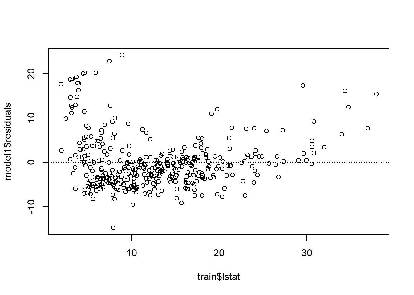
We can also verify linearity using some external libraries.
# Assessing linearity
library(car)
crPlots(model1)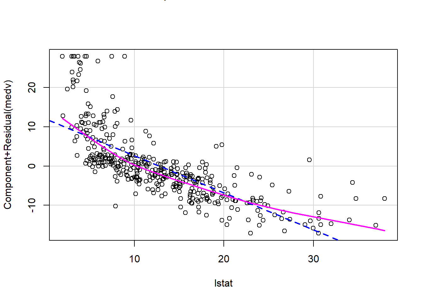
Is there any apparent pattern in the residuals plot?
18.4.2 Nearly normal residuals
To check this condition, we can look at a histogram:
hist(model1$residuals)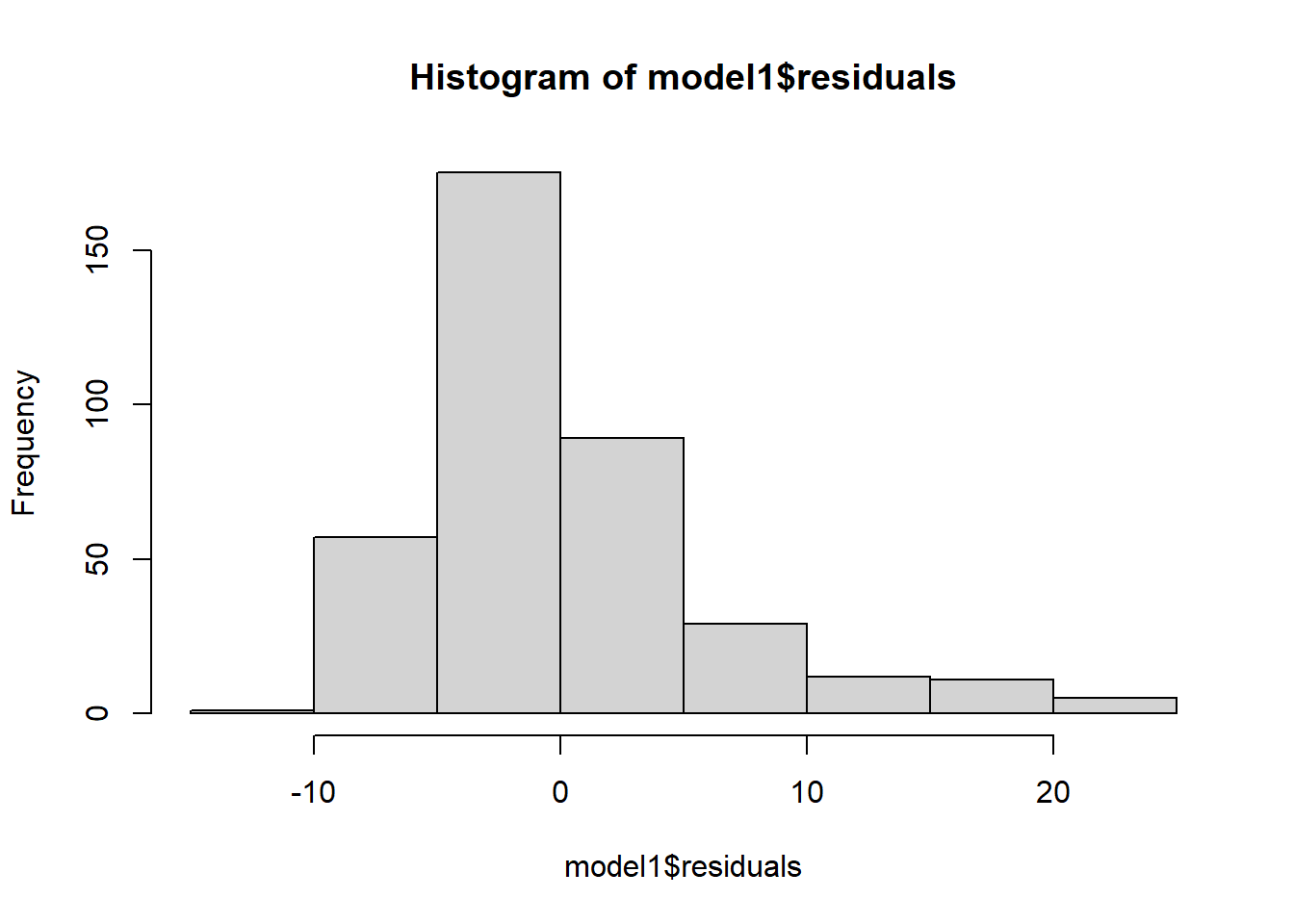
or a normal probability plot of the residuals.
qqnorm(model1$residuals)
qqline(model1$residuals)  # adds diagonal line to the normal prob plot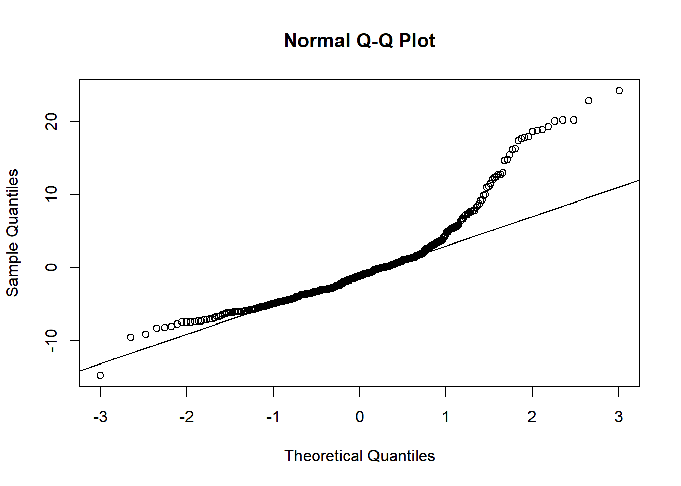
Based on the histogram and the normal probability plot, does the nearly normal residuals condition appear to be met?
18.4.3 Constant variability
# Assessing homoscedasticity
library(car)
ncvTest(model1)
## Non-constant Variance Score Test
## Variance formula: ~ fitted.values
## Chisquare = 23.86532, Df = 1, p = 1.0332e-06spreadLevelPlot(model1)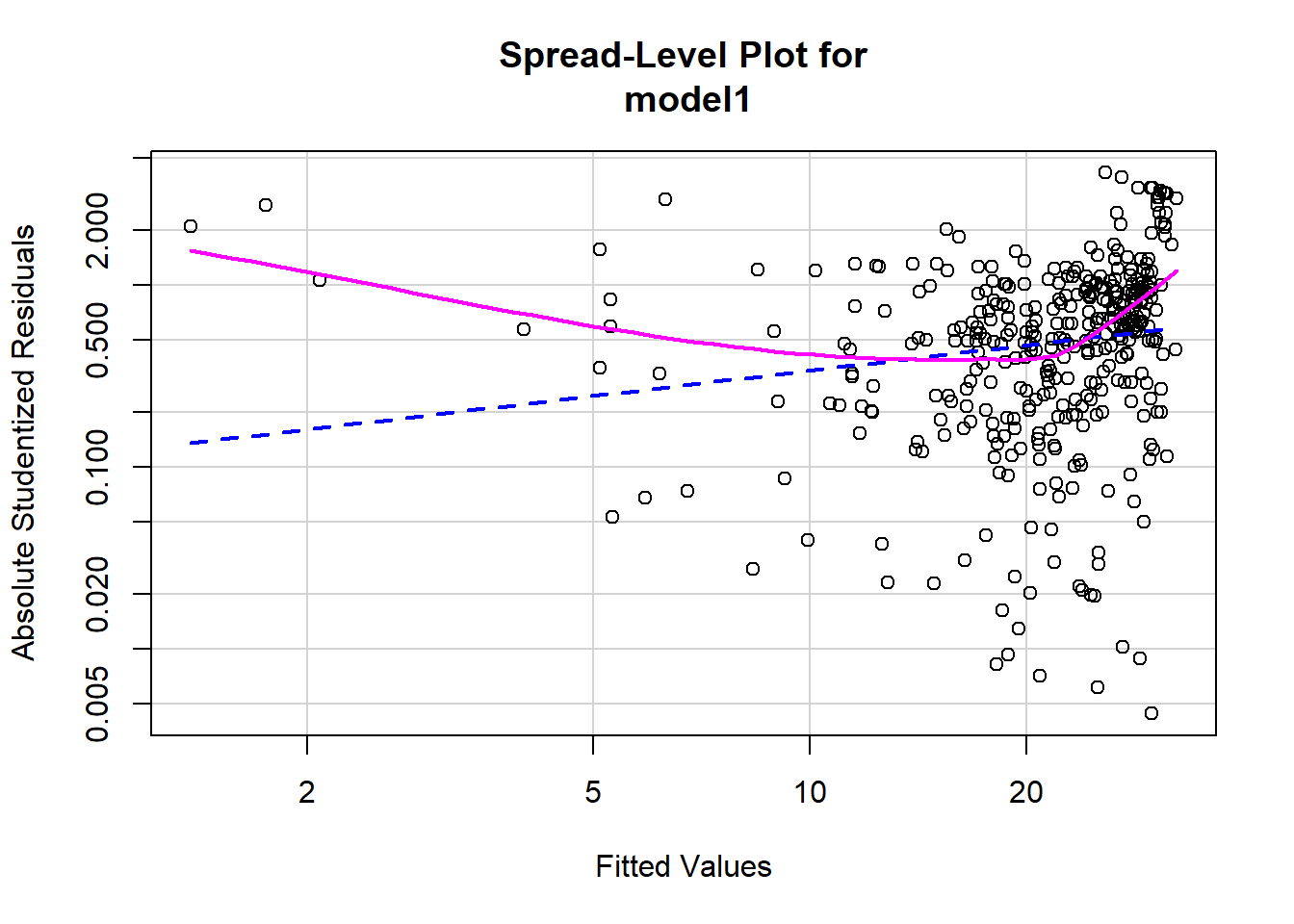
##
## Suggested power transformation:  0.5369863
Based on the plot in (1), does the constant variability condition appear to be met?
18.4.4 Outliers
Outliers observations aren’t predicted well by regression model. They either have extremely large positive or negative residuals. If the model is underestimating the response value, then it will be indicated by positive residual. On the other hand, if the model is overestimating the response value, then it will be indicated by negative residual.
From our regression model example, we can start investigating outliers observation by using Q-Q plot. Code below helps you to plot and find potential outliers.
#install.packages(“car”)
library(car)
qqPlot(model1,labels=row.names(train), id.method="identify",
         simulate=TRUE, main="Q-Q Plot")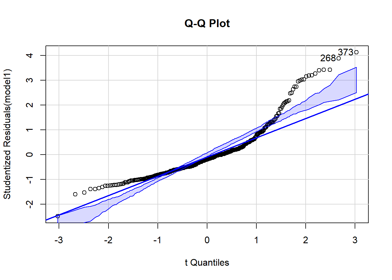
## 373 268
## 124 187
Applying outlierTest function is helping us to confirm if potential outliers are indeed outliers. The statistical test is showing that both cases are undeniably detected as outliers.
outlierTest(model1)## rstudent unadjusted p-value Bonferroni p
## 373 4.127628 4.5175e-05 0.017121
## 268 3.888591 1.1920e-04 0.04517518.4.5 Leverage points
Observations will be considered as high-leverage points if they resemble outliers when we compared it to other predictors. Strictly speaking, they have uncommon combination of predictor values while the response value has minor impact on determining leverage.
You can compute the high leverage observation by looking at the ratio of number of parameters estimated in model and sample size. If an observation has a ratio greater than 2 -3 times the average ratio, then the observation considers as high-leverage points. I
highleverage <- function(fit) {
 p <- length(coefficients(fit))
 n <- length(fitted(fit))
 ratio <-p/n
 plot(hatvalues(fit), main="Index Plot of Ratio")
 abline(h=c(2,3)*ratio, col="red", lty=2)
 identify(1:n, hatvalues(fit), names(hatvalues(fit)))
}
highleverage(model1)
## integer(0)The graph above indicates that we have many observations that have the very high ratio. It means these are quite unusual if we compared their predictor values compared to other.
One thing to remember that not all high-leverage observations are influential observations. It will depend if they are outliers or not.
18.4.6 Influential observations
Observations with a disproportionate impact on the values of the model parameters can be considered as Influential observations. For instance, if you drop a single observation, then it change your model dramatically. That single observation must be influential observation. Thus, it is important for us to inspect if our data contains influential points or not.
Cook’s distance - measures how much the entire regression function changes when the i-th case is deleted. Bar Plot of Cook’s distance to detect observations that strongly influence fitted values of the model.
Cook’s distance was introduced by American statistician R Dennis Cook in 1977. It is used to identify influential data points. It depends on both the residual and leverage i.e it takes it account both the x value and y value of the observation.
Steps to compute Cook’s distance:
delete observations one at a time,
refit the regression model on remaining (n−1)observations,
examine how much all of the fitted values change when the i-th observation is deleted.
A data point having a large cook’s d indicates that the data point strongly influences the fitted values.
ols_plot_cooksd_bar(model1)
I need to highlight that the plot above is indeed helpful to identify influential observations, but it doesn’t give extra information about how these observations affect the model.
That’s why Added Variable plots can be an option for us to dig more information.
Added variable plots works by plotting each predictor variable against the response variable and other predictors. It can be easily created using the avPlots() function in car package.
avPlots(model1, ask=FALSE, id.method="identify")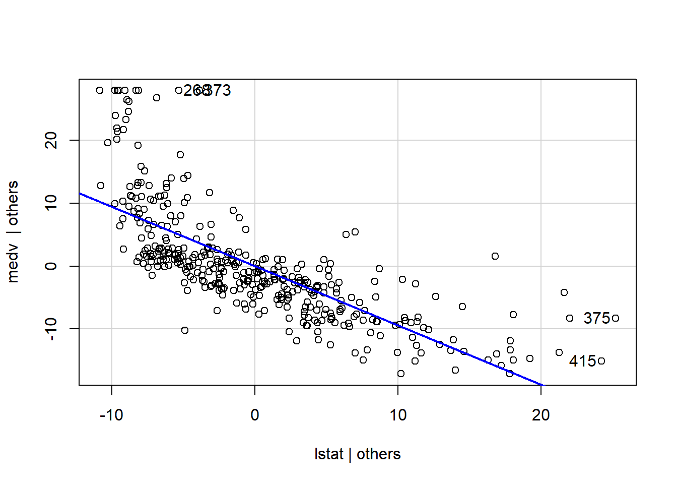
From the graph above, the straight line in each plot is the actual regression coefficient for that predictor variable. We might view the impact of influential observations by imagining how the line would alter if the point representing that observation was removed.
Now, we will incorporate all information from outlier, high-leverage, and influential observations into a single informative plot. I personally find influencePlot() is a very handy function to represent these unusual observation issues.
influencePlot(model1, id.method="identify", main="Influence Plot", sub="Circle size is proportional to Cook’s distance")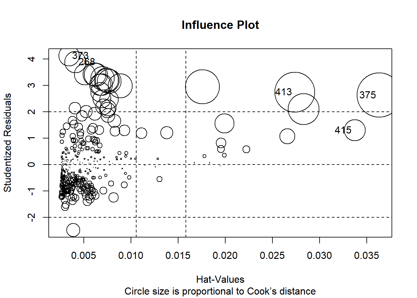
| StudRes | Hat | CookD |
|---|---|---|
| 1.31 | 0.0337 | 0.0297 |
| 4.13 | 0.00343 | 0.0282 |
| 2.64 | 0.0363 | 0.129 |
| 3.89 | 0.00414 | 0.0303 |
| 2.75 | 0.0274 | 0.105 |
So - as we noticed, observations no.: 415; 373; 375; 268 and 413 are problematic. Which of those are influential; leverage or outliers?
18.4.7 Global tests of linear model assumptions
#install.packages("gvlma")
library(gvlma)
gvmodel <- gvlma(model1)
summary(gvmodel)
##
## Call:
## lm(formula = medv ~ lstat, data = train)
##
## Residuals:
## Min 1Q Median 3Q Max
## -14.800 -3.753 -1.161 1.690 24.242
##
## Coefficients:
## Estimate Std. Error t value Pr(>|t|)
## (Intercept) 34.12056 0.63739 53.53 <2e-16 ***
## lstat -0.94171 0.04372 -21.54 <2e-16 ***
## ---
## Signif. codes: 0 '***' 0.001 '**' 0.01 '*' 0.05 '.' 0.1 ' ' 1
##
## Residual standard error: 6.007 on 377 degrees of freedom
## Multiple R-squared: 0.5517, Adjusted R-squared: 0.5505
## F-statistic: 464 on 1 and 377 DF, p-value: < 2.2e-16
##
##
## ASSESSMENT OF THE LINEAR MODEL ASSUMPTIONS
## USING THE GLOBAL TEST ON 4 DEGREES-OF-FREEDOM:
## Level of Significance = 0.05
##
## Call:
## gvlma(x = model1)
##
## Value p-value Decision
## Global Stat 339.212 0.0000 Assumptions NOT satisfied!
## Skewness 146.509 0.0000 Assumptions NOT satisfied!
## Kurtosis 118.408 0.0000 Assumptions NOT satisfied!
## Link Function 73.635 0.0000 Assumptions NOT satisfied!
## Heteroscedasticity 0.659 0.4169 Assumptions acceptable.18.5 Nonlinear regression model
We improve our model by adding non-linear coefficient to our model:
model2=lm(medv~lstat+I(lstat^2),data=train)
summary(model2)
##
## Call:
## lm(formula = medv ~ lstat + I(lstat^2), data = train)
##
## Residuals:
## Min 1Q Median 3Q Max
## -15.0041 -3.8585 -0.6233 2.3328 24.6350
##
## Coefficients:
## Estimate Std. Error t value Pr(>|t|)
## (Intercept) 41.791558 0.988539 42.276 <2e-16 ***
## lstat -2.199963 0.137861 -15.958 <2e-16 ***
## I(lstat^2) 0.039428 0.004141 9.522 <2e-16 ***
## ---
## Signif. codes: 0 '***' 0.001 '**' 0.01 '*' 0.05 '.' 0.1 ' ' 1
##
## Residual standard error: 5.399 on 376 degrees of freedom
## Multiple R-squared: 0.6388, Adjusted R-squared: 0.6369
## F-statistic: 332.5 on 2 and 376 DF, p-value: < 2.2e-16dat <- data.frame(lstat = (1:40), medv = predict(model2, data.frame(lstat = (1:40))))
plot_ly() %>%
add_trace(x=~lstat, y=~medv, type="scatter", mode="lines", data = dat, name = "Predicted Value") %>%
add_trace(x=~lstat, y=~medv, type="scatter", data = test, name = "Actual Value")Please run diagnostics and check the RMSE for this model also.
par(mfrow = c(2,2))
plot(model2)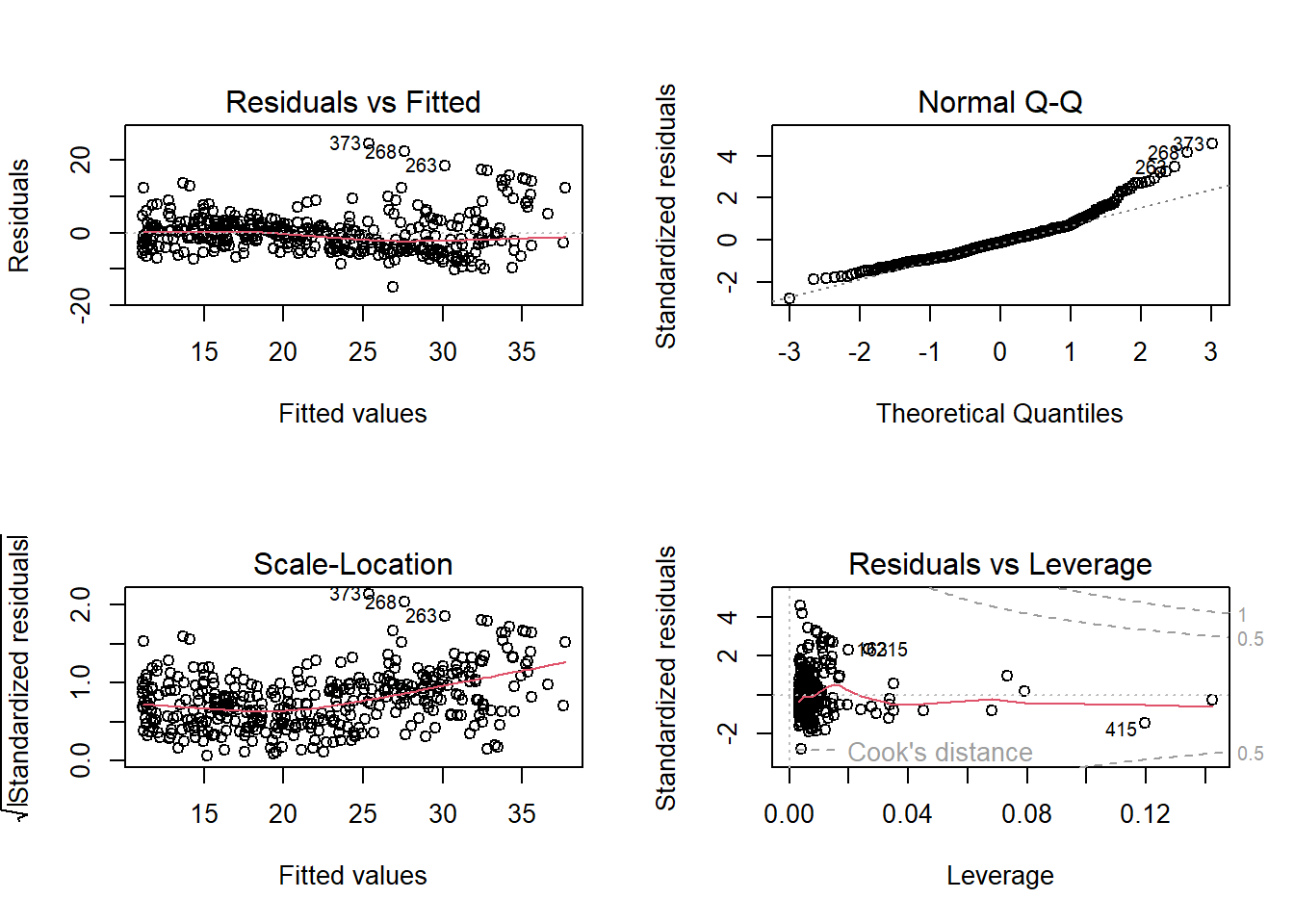
## [1] 5.924323By simply adding non-linear coefficient to our model, the RMSE dropped significantly and the model fitted the data much better. We will continue to improve our model by using other variables as well.
18.6 Multiple variables regression model
In the previous sub-chapters we noticed that we can use correlation matrix to select best variable for our simple model. From that correlation matrix, some of us can deduce that selecting variables for multiple linear regression model can be simple as this:
1. Calculate the correlation matrix of all the predictors
2. Pick the predictor that have a low correlation to each other (to avoid collinearity)
3. Remove the factors that have a low t-stat (large errors)
4. Add other factors (still based on the low correlation factor found in 2.).
**5. Reiterate several times until some criterion (e.g p-value) is over a certain threshold or cannot or we can’t find a larger value.
But unfortunately, THE WHOLE PROCESS MENTIONED ABOVE IS WRONG!!! It is nothing more than p-value hacking.
Gung from stackexchange or kaggle has a very good and detailed explaination why this approach is wrong. I will quote his major points in here.
1. It yields R-squared values that are badly biased to be high.
2. The F and chi-squared tests quoted next to each variable on the printout do not have the claimed distribution.
3. The method yields confidence intervals for effects and predicted values that are falsely narrow; see Altman and Andersen (1989).
4. It yields p-values that do not have the proper meaning, and the proper correction for them is a difficult problem.
5. It gives biased regression coefficients that need shrinkage (the coefficients for remaining variables are too large; see Tibshirani [1996]).
6. It has severe problems in the presence of collinearity.
7. It is based on methods (e.g., F tests for nested models) that were intended to be used to test prespecified hypotheses.
8. Increasing the sample size does not help very much; see Derksen and Keselman (1992).
9. It allows us to not think about the problem.
10. It uses a lot of paper.
Generally, selecting variables for linear regression is a debatable topic.
There are many methods for variable selecting, namely, forward stepwise selection, backward stepwise selection, etc, some are valid, some are heavily criticized.
I recommend this document and Gung’s comment if you want to learn more about variable selection process.
If our goal is prediction, it is safer to include all predictors in our model, removing variables without knowing the science behind it usually does more harm than good!!!
We begin to create our multiple linear regression model:
model3=lm(medv~crim+zn+indus+chas+nox+rm+age+dis+rad+tax+ptratio+black+lstat+I(lstat^2),data=train)
summary(model3)
##
## Call:
## lm(formula = medv ~ crim + zn + indus + chas + nox + rm + age +
## dis + rad + tax + ptratio + black + lstat + I(lstat^2), data = train)
##
## Residuals:
## Min 1Q Median 3Q Max
## -15.5528 -2.3805 -0.3195 1.7342 24.7913
##
## Coefficients:
## Estimate Std. Error t value Pr(>|t|)
## (Intercept) 43.799421 5.151894 8.502 4.89e-16 ***
## crim -0.135197 0.030422 -4.444 1.17e-05 ***
## zn 0.024778 0.014222 1.742 0.082318 .
## indus 0.043005 0.060892 0.706 0.480485
## chas 2.213046 0.889561 2.488 0.013301 *
## nox -19.393777 4.040227 -4.800 2.32e-06 ***
## rm 3.329732 0.448026 7.432 7.71e-13 ***
## age 0.021802 0.013471 1.618 0.106438
## dis -1.187884 0.214759 -5.531 6.08e-08 ***
## rad 0.334585 0.069606 4.807 2.25e-06 ***
## tax -0.014200 0.003915 -3.627 0.000328 ***
## ptratio -0.863652 0.130906 -6.598 1.48e-10 ***
## black 0.006460 0.002552 2.531 0.011787 *
## lstat -1.504056 0.143232 -10.501 < 2e-16 ***
## I(lstat^2) 0.029150 0.003678 7.925 2.82e-14 ***
## ---
## Signif. codes: 0 '***' 0.001 '**' 0.01 '*' 0.05 '.' 0.1 ' ' 1
##
## Residual standard error: 4.156 on 364 degrees of freedom
## Multiple R-squared: 0.7928, Adjusted R-squared: 0.7848
## F-statistic: 99.47 on 14 and 364 DF, p-value: < 2.2e-16We can also construct our model using ~
model4 <- lm(medv ~ ., data = train)
summary(model4)
##
## Call:
## lm(formula = medv ~ ., data = train)
##
## Residuals:
## Min 1Q Median 3Q Max
## -13.5961 -2.6535 -0.4528 1.5304 27.8964
##
## Coefficients:
## Estimate Std. Error t value Pr(>|t|)
## (Intercept) 39.922825 5.545823 7.199 3.49e-12 ***
## crim -0.100314 0.032551 -3.082 0.002214 **
## zn 0.047054 0.015076 3.121 0.001945 **
## indus 0.013327 0.065721 0.203 0.839418
## chas 2.366491 0.961698 2.461 0.014327 *
## nox -22.368843 4.349992 -5.142 4.44e-07 ***
## rm 3.861369 0.479010 8.061 1.09e-14 ***
## age -0.003438 0.014154 -0.243 0.808217
## dis -1.524517 0.227641 -6.697 8.06e-11 ***
## rad 0.356961 0.075206 4.746 2.98e-06 ***
## tax -0.015700 0.004229 -3.713 0.000237 ***
## ptratio -0.974336 0.140747 -6.923 2.00e-11 ***
## black 0.007374 0.002757 2.675 0.007815 **
## lstat -0.450427 0.057607 -7.819 5.77e-14 ***
## ---
## Signif. codes: 0 '***' 0.001 '**' 0.01 '*' 0.05 '.' 0.1 ' ' 1
##
## Residual standard error: 4.495 on 365 degrees of freedom
## Multiple R-squared: 0.757, Adjusted R-squared: 0.7484
## F-statistic: 87.48 on 13 and 365 DF, p-value: < 2.2e-16Looking at model summary, we see that variables indus and age are insignificant, so let’s estimate the model without variables indus and age:
model5 <- lm(medv ~ . -indus -age, data = train)
summary(model5)
##
## Call:
## lm(formula = medv ~ . - indus - age, data = train)
##
## Residuals:
## Min 1Q Median 3Q Max
## -13.5425 -2.6342 -0.4571 1.5392 27.7602
##
## Coefficients:
## Estimate Std. Error t value Pr(>|t|)
## (Intercept) 40.055298 5.489956 7.296 1.84e-12 ***
## crim -0.100670 0.032441 -3.103 0.00206 **
## zn 0.046957 0.014782 3.177 0.00162 **
## chas 2.377649 0.956061 2.487 0.01333 *
## nox -22.475532 3.957782 -5.679 2.76e-08 ***
## rm 3.827429 0.465063 8.230 3.31e-15 ***
## dis -1.518396 0.214033 -7.094 6.75e-12 ***
## rad 0.355574 0.072176 4.926 1.27e-06 ***
## tax -0.015392 0.003888 -3.959 9.05e-05 ***
## ptratio -0.974680 0.139224 -7.001 1.22e-11 ***
## black 0.007320 0.002744 2.667 0.00799 **
## lstat -0.454704 0.053377 -8.519 4.22e-16 ***
## ---
## Signif. codes: 0 '***' 0.001 '**' 0.01 '*' 0.05 '.' 0.1 ' ' 1
##
## Residual standard error: 4.483 on 367 degrees of freedom
## Multiple R-squared: 0.757, Adjusted R-squared: 0.7497
## F-statistic: 103.9 on 11 and 367 DF, p-value: < 2.2e-16Summary of model 5 shows that all variables are significant (based on p-value).
Let’s take a look if there is no multicollinearity problem between predictors.
18.7 Evaluating multi-collinearity
There are many standards researchers apply for deciding whether a VIF is too large.
In some domains, a VIF over 2 is worthy of suspicion.
Others set the bar higher, at 5 or 10.
Others still will say you shouldn’t pay attention to these at all. Ultimately, the main thing to consider is that small effects are more likely to be drowned out by higher VIFs, but this may just be a natural, unavoidable fact with your model.
library(car)
vif(model5)
## crim zn chas nox rm dis rad tax
## 1.743802 2.253607 1.062069 3.776591 1.861788 3.557103 7.709634 8.208439
## ptratio black lstat
## 1.717380 1.376717 2.676471sqrt(vif(model5)) > 2 # problem?## crim zn chas nox rm dis rad tax ptratio black
## FALSE FALSE FALSE FALSE FALSE FALSE TRUE TRUE FALSE FALSE
## lstat
## FALSEFinally we test our model on test dataset:
evaluate<-predict(model5, test)
rmse(evaluate,test[,14 ])
## [1] 5.56882518.8 Best subset regression
Best subset (13 variable) and stepwise (forward, backward, both) techniques of variable selection can be used to come up with the best linear regression model for the dependent variable medv.
The R function regsubsets() [leaps package] can be used to identify different best models of different sizes.
Ideally we would test every possible combination of covariates and use the combination with the best performance. This is best subset selection.
Consider the case of three covariates: X1, X2, and X3. We would estimate the accuracy of the following models:
- All variables: X1, X2, X3 - our default regression
- X1 and X2 (exclude X3)
- X2 and X3 (exclude X1)
- X1 and X3 (exclude X2)
- X1-only
- X2-only
- X3-only
- No variables (intercept only)
The one with the best performance (e.g. cross-validated mean-squared error) is the one we would use. Stepwise algorithms are commonly used without cross-validation, and as a result they are usually overfitting the data - capturing random error in addition to true relationships in the data, resulting in worse performance on new data.
To generalize to any model size, if we have p covariates we would have to check \(2^p\) different combinations: each covariate is either included or not (2 possibilities), so combining that for all covariates we have the product of p twos: \(2 * 2 * 2...\) which simplifies to \(2^p\). With 10 covariates that is 1,024 models to check, with 20 covariates it’s a million, etc.
You need to specify the option nvmax, which represents the maximum number of predictors to incorporate in the model.
For example, if nvmax = 5, the function will return up to the best 5-variables model, that is, it returns the best 1-variable model, the best 2-variables model, …, the best 5-variables models.
In our example, we have 13 predictor variables in the data.
So, we’ll use nvmax = 13.
model.subset <- regsubsets(medv ~ ., data = train, nbest = 1, nvmax = 13)
summary(model.subset)
## Subset selection object
## Call: regsubsets.formula(medv ~ ., data = train, nbest = 1, nvmax = 13)
## 13 Variables (and intercept)
## Forced in Forced out
## crim FALSE FALSE
## zn FALSE FALSE
## indus FALSE FALSE
## chas FALSE FALSE
## nox FALSE FALSE
## rm FALSE FALSE
## age FALSE FALSE
## dis FALSE FALSE
## rad FALSE FALSE
## tax FALSE FALSE
## ptratio FALSE FALSE
## black FALSE FALSE
## lstat FALSE FALSE
## 1 subsets of each size up to 13
## Selection Algorithm: exhaustive
## crim zn indus chas nox rm age dis rad tax ptratio black lstat
## 1 ( 1 ) " " " " " " " " " " " " " " " " " " " " " " " " "*"
## 2 ( 1 ) " " " " " " " " " " "*" " " " " " " " " " " " " "*"
## 3 ( 1 ) " " " " " " " " " " "*" " " " " " " " " "*" " " "*"
## 4 ( 1 ) " " " " " " " " " " "*" " " " " " " " " "*" "*" "*"
## 5 ( 1 ) " " " " " " " " "*" "*" " " "*" " " " " "*" " " "*"
## 6 ( 1 ) " " " " " " "*" "*" "*" " " "*" " " " " "*" " " "*"
## 7 ( 1 ) " " " " " " "*" "*" "*" " " "*" " " " " "*" "*" "*"
## 8 ( 1 ) "*" " " " " " " "*" "*" " " "*" "*" "*" "*" " " "*"
## 9 ( 1 ) "*" "*" " " " " "*" "*" " " "*" "*" "*" "*" " " "*"
## 10 ( 1 ) "*" "*" " " " " "*" "*" " " "*" "*" "*" "*" "*" "*"
## 11 ( 1 ) "*" "*" " " "*" "*" "*" " " "*" "*" "*" "*" "*" "*"
## 12 ( 1 ) "*" "*" " " "*" "*" "*" "*" "*" "*" "*" "*" "*" "*"
## 13 ( 1 ) "*" "*" "*" "*" "*" "*" "*" "*" "*" "*" "*" "*" "*"plot(model.subset, scale = "bic")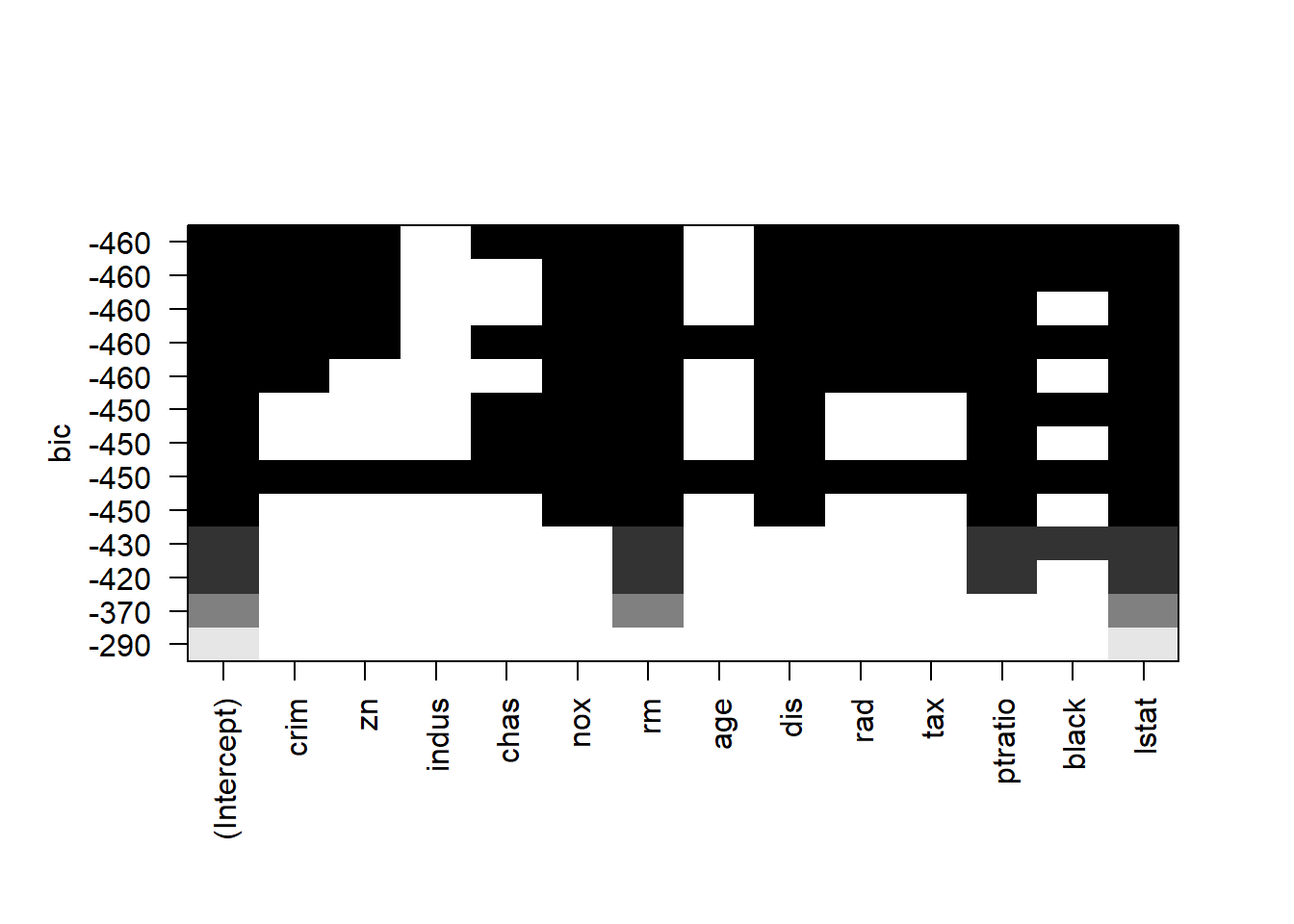
18.9 Stepwise regression
Stepwise selection, or stepwise regression, is a commonly used technique to include a subset of covariates in a regression model.
The goal is to increase accuracy compared to including all covariates in the model, because we can often improve model performance by removing some covariates (as we did with lasso / elastic net). Stepwise is a simple form of feature selection - choosing a subset of variables for incorporation into a machine learning algorithm.
Stepwise selection is a simplification of best subset selection to make it computationally feasible for any number of covariates. It comes in three forms: forward, backward, and combined forward & backward. Confusingly, sometimes “stepwise” is meant to refer specifically to the “both” approach.
Forward selection starts with just the intercept and considers which single variable to incorporate next. It loops over every variable, runs a regression with that variable plus the intercept, and chooses the variable with the best performance on a certain metric: adjusted \(R^2\), f-statistic, Aikake Information Criterion, or other preferred performance estimate. It then adds that variable to the model and considers the next variable to add, continuing to repeat until no remaining variable improves performance.
nullmodel <- lm(medv ~ 1, data = train)
fullmodel <- lm(medv ~ ., data = train)

#forward selection
model_forward <- step(nullmodel, scope = list(lower = nullmodel, upper = fullmodel), direction = "forward")
## Start: AIC=1663.11
## medv ~ 1
##
## Df Sum of Sq RSS AIC
## + lstat 1 16742.0 13604 1361.0
## + rm 1 14646.4 15699 1415.3
## + ptratio 1 9548.3 20797 1521.9
## + indus 1 8198.9 22147 1545.7
## + tax 1 8158.8 22187 1546.4
## + nox 1 6384.0 23962 1575.6
## + rad 1 5797.6 24548 1584.8
## + age 1 5288.0 25058 1592.5
## + crim 1 5042.1 25304 1596.2
## + zn 1 4923.7 25422 1598.0
## + black 1 3711.3 26634 1615.7
## + dis 1 2631.0 27715 1630.7
## + chas 1 757.8 29588 1655.5
## <none> 30346 1663.1
##
## Step: AIC=1361.03
## medv ~ lstat
##
## Df Sum of Sq RSS AIC
## + rm 1 2768.88 10835 1276.8
## + ptratio 1 1955.30 11648 1304.2
## + chas 1 451.45 13152 1350.2
## + tax 1 380.94 13223 1352.3
## + indus 1 269.35 13334 1355.5
## + zn 1 263.37 13340 1355.6
## + dis 1 236.76 13367 1356.4
## + black 1 150.31 13453 1358.8
## + crim 1 117.90 13486 1359.7
## + nox 1 91.82 13512 1360.5
## <none> 13604 1361.0
## + rad 1 55.10 13549 1361.5
## + age 1 33.39 13570 1362.1
##
## Step: AIC=1276.78
## medv ~ lstat + rm
##
## Df Sum of Sq RSS AIC
## + ptratio 1 1412.72 9422.1 1225.8
## + tax 1 634.44 10200.4 1255.9
## + black 1 334.07 10500.7 1266.9
## + chas 1 317.48 10517.3 1267.5
## + rad 1 289.40 10545.4 1268.5
## + crim 1 258.28 10576.5 1269.6
## + nox 1 257.10 10577.7 1269.7
## + indus 1 236.22 10598.6 1270.4
## + zn 1 121.62 10713.2 1274.5
## <none> 10834.8 1276.8
## + dis 1 46.19 10788.6 1277.2
## + age 1 29.56 10805.3 1277.8
##
## Step: AIC=1225.83
## medv ~ lstat + rm + ptratio
##
## Df Sum of Sq RSS AIC
## + black 1 299.071 9123.0 1215.6
## + nox 1 253.469 9168.6 1217.5
## + tax 1 206.601 9215.5 1219.4
## + chas 1 173.996 9248.1 1220.8
## + crim 1 142.872 9279.2 1222.0
## + dis 1 83.386 9338.7 1224.5
## + indus 1 77.535 9344.6 1224.7
## <none> 9422.1 1225.8
## + rad 1 23.953 9398.1 1226.9
## + age 1 10.036 9412.1 1227.4
## + zn 1 3.428 9418.7 1227.7
##
## Step: AIC=1215.61
## medv ~ lstat + rm + ptratio + black
##
## Df Sum of Sq RSS AIC
## + chas 1 159.895 8963.1 1210.9
## + nox 1 142.903 8980.1 1211.6
## + dis 1 137.857 8985.2 1211.8
## + tax 1 81.863 9041.2 1214.2
## + crim 1 68.267 9054.8 1214.8
## <none> 9123.0 1215.6
## + indus 1 27.774 9095.3 1216.5
## + age 1 4.715 9118.3 1217.4
## + zn 1 1.619 9121.4 1217.5
## + rad 1 1.213 9121.8 1217.6
##
## Step: AIC=1210.91
## medv ~ lstat + rm + ptratio + black + chas
##
## Df Sum of Sq RSS AIC
## + nox 1 192.347 8770.8 1204.7
## + dis 1 105.326 8857.8 1208.4
## + tax 1 81.779 8881.4 1209.4
## + crim 1 61.620 8901.5 1210.3
## <none> 8963.1 1210.9
## + indus 1 46.927 8916.2 1210.9
## + age 1 12.826 8950.3 1212.4
## + zn 1 5.271 8957.9 1212.7
## + rad 1 0.432 8962.7 1212.9
##
## Step: AIC=1204.68
## medv ~ lstat + rm + ptratio + black + chas + nox
##
## Df Sum of Sq RSS AIC
## + dis 1 709.91 8060.9 1174.7
## + rad 1 64.92 8705.9 1203.9
## <none> 8770.8 1204.7
## + crim 1 31.03 8739.7 1205.3
## + age 1 30.90 8739.9 1205.3
## + zn 1 12.11 8758.7 1206.2
## + indus 1 6.96 8763.8 1206.4
## + tax 1 3.88 8766.9 1206.5
##
## Step: AIC=1174.69
## medv ~ lstat + rm + ptratio + black + chas + nox + dis
##
## Df Sum of Sq RSS AIC
## + zn 1 120.907 7940.0 1171.0
## + rad 1 107.158 7953.7 1171.6
## + crim 1 48.055 8012.8 1174.4
## <none> 8060.9 1174.7
## + indus 1 23.453 8037.4 1175.6
## + age 1 21.767 8039.1 1175.7
## + tax 1 0.028 8060.8 1176.7
##
## Step: AIC=1170.97
## medv ~ lstat + rm + ptratio + black + chas + nox + dis + zn
##
## Df Sum of Sq RSS AIC
## + crim 1 76.511 7863.5 1169.3
## + rad 1 75.216 7864.7 1169.4
## <none> 7940.0 1171.0
## + indus 1 18.678 7921.3 1172.1
## + age 1 10.838 7929.1 1172.5
## + tax 1 9.355 7930.6 1172.5
##
## Step: AIC=1169.3
## medv ~ lstat + rm + ptratio + black + chas + nox + dis + zn +
## crim
##
## Df Sum of Sq RSS AIC
## + rad 1 173.071 7690.4 1162.9
## <none> 7863.5 1169.3
## + indus 1 18.847 7844.6 1170.4
## + age 1 14.724 7848.7 1170.6
## + tax 1 0.243 7863.2 1171.3
##
## Step: AIC=1162.86
## medv ~ lstat + rm + ptratio + black + chas + nox + dis + zn +
## crim + rad
##
## Df Sum of Sq RSS AIC
## + tax 1 314.923 7375.5 1149.0
## <none> 7690.4 1162.9
## + indus 1 35.945 7654.4 1163.1
## + age 1 2.384 7688.0 1164.7
##
## Step: AIC=1149.02
## medv ~ lstat + rm + ptratio + black + chas + nox + dis + zn +
## crim + rad + tax
##
## Df Sum of Sq RSS AIC
## <none> 7375.5 1149
## + age 1 1.23685 7374.2 1151
## + indus 1 0.87563 7374.6 1151Backward selection does the same thing but it starts with all variables in the model and considers which variable to first remove from the model. It checks the performance for each variable when it is removed and removes the variable that is least useful to the regression performance. It continues this until no variable yields an increase in performance upon removal.
Challenges
- How similar are stepwise results compared to the significant covariates from the standard OLS we ran first? Hint: compare
step_regwithsummary(largest_model). - Try running with
trace = 1to see more details in the stepwise process. - Try running with
direction = "backward"and thendirection = "both"- do you get the same variables selected? Hint: with backward you will need to change the first argument to use the full model rather than the intercept-only model.
#Backward selection
model.backward <- step(fullmodel, direction = "backward")
## Start: AIC=1152.91
## medv ~ crim + zn + indus + chas + nox + rm + age + dis + rad +
## tax + ptratio + black + lstat
##
## Df Sum of Sq RSS AIC
## - indus 1 0.83 7374.2 1151.0
## - age 1 1.19 7374.6 1151.0
## <none> 7373.4 1152.9
## - chas 1 122.32 7495.7 1157.1
## - black 1 144.52 7517.9 1158.3
## - crim 1 191.86 7565.3 1160.6
## - zn 1 196.80 7570.2 1160.9
## - tax 1 278.45 7651.8 1165.0
## - rad 1 455.10 7828.5 1173.6
## - nox 1 534.18 7907.6 1177.4
## - dis 1 906.02 8279.4 1194.8
## - ptratio 1 968.09 8341.5 1197.7
## - lstat 1 1235.03 8608.4 1209.6
## - rm 1 1312.71 8686.1 1213.0
##
## Step: AIC=1150.95
## medv ~ crim + zn + chas + nox + rm + age + dis + rad + tax +
## ptratio + black + lstat
##
## Df Sum of Sq RSS AIC
## - age 1 1.24 7375.5 1149.0
## <none> 7374.2 1151.0
## - chas 1 124.70 7498.9 1155.3
## - black 1 143.94 7518.2 1156.3
## - crim 1 193.07 7567.3 1158.8
## - zn 1 197.55 7571.8 1159.0
## - tax 1 313.78 7688.0 1164.7
## - rad 1 473.55 7847.8 1172.5
## - nox 1 561.95 7936.2 1176.8
## - dis 1 953.67 8327.9 1195.0
## - ptratio 1 971.37 8345.6 1195.8
## - lstat 1 1237.30 8611.5 1207.7
## - rm 1 1318.35 8692.6 1211.3
##
## Step: AIC=1149.02
## medv ~ crim + zn + chas + nox + rm + dis + rad + tax + ptratio +
## black + lstat
##
## Df Sum of Sq RSS AIC
## <none> 7375.5 1149.0
## - chas 1 124.29 7499.8 1153.3
## - black 1 142.95 7518.4 1154.3
## - crim 1 193.53 7569.0 1156.8
## - zn 1 202.81 7578.3 1157.3
## - tax 1 314.92 7690.4 1162.9
## - rad 1 487.75 7863.2 1171.3
## - nox 1 648.10 8023.6 1178.9
## - ptratio 1 984.97 8360.4 1194.5
## - dis 1 1011.42 8386.9 1195.7
## - rm 1 1361.18 8736.6 1211.2
## - lstat 1 1458.37 8833.8 1215.4#stepwise selection
model.step <- step(nullmodel, scope = list(lower = nullmodel, upper = fullmodel), direction = "both")## Start: AIC=1663.11
## medv ~ 1
##
## Df Sum of Sq RSS AIC
## + lstat 1 16742.0 13604 1361.0
## + rm 1 14646.4 15699 1415.3
## + ptratio 1 9548.3 20797 1521.9
## + indus 1 8198.9 22147 1545.7
## + tax 1 8158.8 22187 1546.4
## + nox 1 6384.0 23962 1575.6
## + rad 1 5797.6 24548 1584.8
## + age 1 5288.0 25058 1592.5
## + crim 1 5042.1 25304 1596.2
## + zn 1 4923.7 25422 1598.0
## + black 1 3711.3 26634 1615.7
## + dis 1 2631.0 27715 1630.7
## + chas 1 757.8 29588 1655.5
## <none> 30346 1663.1
##
## Step: AIC=1361.03
## medv ~ lstat
##
## Df Sum of Sq RSS AIC
## + rm 1 2768.9 10835 1276.8
## + ptratio 1 1955.3 11648 1304.2
## + chas 1 451.5 13152 1350.2
## + tax 1 380.9 13223 1352.3
## + indus 1 269.3 13334 1355.5
## + zn 1 263.4 13340 1355.6
## + dis 1 236.8 13367 1356.4
## + black 1 150.3 13453 1358.8
## + crim 1 117.9 13486 1359.7
## + nox 1 91.8 13512 1360.5
## <none> 13604 1361.0
## + rad 1 55.1 13549 1361.5
## + age 1 33.4 13570 1362.1
## - lstat 1 16742.0 30346 1663.1
##
## Step: AIC=1276.78
## medv ~ lstat + rm
##
## Df Sum of Sq RSS AIC
## + ptratio 1 1412.7 9422.1 1225.8
## + tax 1 634.4 10200.4 1255.9
## + black 1 334.1 10500.7 1266.9
## + chas 1 317.5 10517.3 1267.5
## + rad 1 289.4 10545.4 1268.5
## + crim 1 258.3 10576.5 1269.6
## + nox 1 257.1 10577.7 1269.7
## + indus 1 236.2 10598.6 1270.4
## + zn 1 121.6 10713.2 1274.5
## <none> 10834.8 1276.8
## + dis 1 46.2 10788.6 1277.2
## + age 1 29.6 10805.3 1277.8
## - rm 1 2768.9 13603.7 1361.0
## - lstat 1 4864.4 15699.3 1415.3
##
## Step: AIC=1225.83
## medv ~ lstat + rm + ptratio
##
## Df Sum of Sq RSS AIC
## + black 1 299.07 9123.0 1215.6
## + nox 1 253.47 9168.6 1217.5
## + tax 1 206.60 9215.5 1219.4
## + chas 1 174.00 9248.1 1220.8
## + crim 1 142.87 9279.2 1222.0
## + dis 1 83.39 9338.7 1224.5
## + indus 1 77.54 9344.6 1224.7
## <none> 9422.1 1225.8
## + rad 1 23.95 9398.1 1226.9
## + age 1 10.04 9412.1 1227.4
## + zn 1 3.43 9418.7 1227.7
## - ptratio 1 1412.72 10834.8 1276.8
## - rm 1 2226.30 11648.4 1304.2
## - lstat 1 3027.35 12449.4 1329.4
##
## Step: AIC=1215.61
## medv ~ lstat + rm + ptratio + black
##
## Df Sum of Sq RSS AIC
## + chas 1 159.89 8963.1 1210.9
## + nox 1 142.90 8980.1 1211.6
## + dis 1 137.86 8985.2 1211.8
## + tax 1 81.86 9041.2 1214.2
## + crim 1 68.27 9054.8 1214.8
## <none> 9123.0 1215.6
## + indus 1 27.77 9095.3 1216.5
## + age 1 4.72 9118.3 1217.4
## + zn 1 1.62 9121.4 1217.5
## + rad 1 1.21 9121.8 1217.6
## - black 1 299.07 9422.1 1225.8
## - ptratio 1 1377.72 10500.7 1266.9
## - lstat 1 2073.53 11196.6 1291.2
## - rm 1 2386.83 11509.9 1301.7
##
## Step: AIC=1210.91
## medv ~ lstat + rm + ptratio + black + chas
##
## Df Sum of Sq RSS AIC
## + nox 1 192.35 8770.8 1204.7
## + dis 1 105.33 8857.8 1208.4
## + tax 1 81.78 8881.4 1209.4
## + crim 1 61.62 8901.5 1210.3
## <none> 8963.1 1210.9
## + indus 1 46.93 8916.2 1210.9
## + age 1 12.83 8950.3 1212.4
## + zn 1 5.27 8957.9 1212.7
## + rad 1 0.43 8962.7 1212.9
## - chas 1 159.89 9123.0 1215.6
## - black 1 284.97 9248.1 1220.8
## - ptratio 1 1242.15 10205.3 1258.1
## - lstat 1 2125.36 11088.5 1289.5
## - rm 1 2315.93 11279.1 1296.0
##
## Step: AIC=1204.68
## medv ~ lstat + rm + ptratio + black + chas + nox
##
## Df Sum of Sq RSS AIC
## + dis 1 709.91 8060.9 1174.7
## + rad 1 64.92 8705.9 1203.9
## <none> 8770.8 1204.7
## + crim 1 31.03 8739.7 1205.3
## + age 1 30.90 8739.9 1205.3
## + zn 1 12.11 8758.7 1206.2
## + indus 1 6.96 8763.8 1206.4
## + tax 1 3.88 8766.9 1206.5
## - black 1 162.12 8932.9 1209.6
## - nox 1 192.35 8963.1 1210.9
## - chas 1 209.34 8980.1 1211.6
## - ptratio 1 1228.23 9999.0 1252.4
## - lstat 1 1293.30 10064.1 1254.8
## - rm 1 2415.58 11186.4 1294.9
##
## Step: AIC=1174.69
## medv ~ lstat + rm + ptratio + black + chas + nox + dis
##
## Df Sum of Sq RSS AIC
## + zn 1 120.91 7940.0 1171.0
## + rad 1 107.16 7953.7 1171.6
## + crim 1 48.05 8012.8 1174.4
## <none> 8060.9 1174.7
## + indus 1 23.45 8037.4 1175.6
## + age 1 21.77 8039.1 1175.7
## + tax 1 0.03 8060.8 1176.7
## - black 1 136.25 8197.1 1179.0
## - chas 1 181.00 8241.9 1181.1
## - dis 1 709.91 8770.8 1204.7
## - nox 1 796.93 8857.8 1208.4
## - ptratio 1 1386.74 9447.6 1232.9
## - lstat 1 1565.73 9626.6 1240.0
## - rm 1 2061.82 10122.7 1259.0
##
## Step: AIC=1170.97
## medv ~ lstat + rm + ptratio + black + chas + nox + dis + zn
##
## Df Sum of Sq RSS AIC
## + crim 1 76.51 7863.5 1169.3
## + rad 1 75.22 7864.7 1169.4
## <none> 7940.0 1171.0
## + indus 1 18.68 7921.3 1172.1
## + age 1 10.84 7929.1 1172.5
## + tax 1 9.35 7930.6 1172.5
## - zn 1 120.91 8060.9 1174.7
## - black 1 151.96 8091.9 1176.2
## - chas 1 183.64 8123.6 1177.6
## - nox 1 806.44 8746.4 1205.6
## - dis 1 818.70 8758.7 1206.2
## - ptratio 1 1095.33 9035.3 1217.9
## - lstat 1 1615.22 9555.2 1239.2
## - rm 1 1781.53 9721.5 1245.7
##
## Step: AIC=1169.3
## medv ~ lstat + rm + ptratio + black + chas + nox + dis + zn +
## crim
##
## Df Sum of Sq RSS AIC
## + rad 1 173.07 7690.4 1162.9
## <none> 7863.5 1169.3
## + indus 1 18.85 7844.6 1170.4
## + age 1 14.72 7848.7 1170.6
## - crim 1 76.51 7940.0 1171.0
## + tax 1 0.24 7863.2 1171.3
## - black 1 112.89 7976.3 1172.7
## - zn 1 149.36 8012.8 1174.4
## - chas 1 169.41 8032.9 1175.4
## - nox 1 755.13 8618.6 1202.0
## - dis 1 867.98 8731.4 1207.0
## - ptratio 1 998.48 8861.9 1212.6
## - lstat 1 1396.14 9259.6 1229.2
## - rm 1 1806.08 9669.5 1245.7
##
## Step: AIC=1162.86
## medv ~ lstat + rm + ptratio + black + chas + nox + dis + zn +
## crim + rad
##
## Df Sum of Sq RSS AIC
## + tax 1 314.92 7375.5 1149.0
## <none> 7690.4 1162.9
## + indus 1 35.94 7654.4 1163.1
## + age 1 2.38 7688.0 1164.7
## - zn 1 114.24 7804.6 1166.5
## - black 1 168.48 7858.9 1169.1
## - chas 1 172.25 7862.6 1169.3
## - rad 1 173.07 7863.5 1169.3
## - crim 1 174.37 7864.7 1169.4
## - dis 1 901.45 8591.8 1202.9
## - nox 1 927.66 8618.0 1204.0
## - ptratio 1 1171.53 8861.9 1214.6
## - lstat 1 1484.66 9175.0 1227.8
## - rm 1 1594.42 9284.8 1232.3
##
## Step: AIC=1149.02
## medv ~ lstat + rm + ptratio + black + chas + nox + dis + zn +
## crim + rad + tax
##
## Df Sum of Sq RSS AIC
## <none> 7375.5 1149.0
## + age 1 1.24 7374.2 1151.0
## + indus 1 0.88 7374.6 1151.0
## - chas 1 124.29 7499.8 1153.3
## - black 1 142.95 7518.4 1154.3
## - crim 1 193.53 7569.0 1156.8
## - zn 1 202.81 7578.3 1157.3
## - tax 1 314.92 7690.4 1162.9
## - rad 1 487.75 7863.2 1171.3
## - nox 1 648.10 8023.6 1178.9
## - ptratio 1 984.97 8360.4 1194.5
## - dis 1 1011.42 8386.9 1195.7
## - rm 1 1361.18 8736.6 1211.2
## - lstat 1 1458.37 8833.8 1215.418.10 Comparing competing models
18.10.1 Akaike Information Criterion
There are numerous model selection criteria based on mathematical information theory that we can use to select models from among a set of candidate models. They additionally allow the relative weights of different models to be compared and allow multiple models to be used for inferences. The most commonly used information criteria in ecology and evolution are: Akaike’s Information Criterion (AIC), the corrected AICc (corrected for small sample sizes), and the Bayesian Information Criterion (BIC, also known as the Schwarz Criterion) (Johnson and Omland, 2004). Here we will focus on AIC and AICc. Here is how AIC is calculated:
\[ AIC = -2Log\mathcal{L} \ + \ 2p \] The lower the AIC value, the better the model. \(-2Log\mathcal{L}\) is called the negative log likelihood of the model, and measures the model’s fit (or lack thereof) to the observed data: Lower negative log-likelihood values indicate a beter fit of the model to the observed data. \(2p\) is a bias correcting factor that penalizes the model AIC based on the number of parameters (p) in the model.
Similar to AIC is AICc, which corrects for small sample sizes. It is recommended to use AICc when \(n/k\) is less than 40, with \(n\) being the sample size (i.e. total number of observations) and \(k\) being the total number of parameters in the most saturated model (i.e. the model with the most parameters), including both fixed and random effects, as well as intercepts (Symonds and Moussalli 2011). AICc is calculated as follows:
\[ AIC_c = AIC+\frac{2k(k+1)}{n-k-1} \]
18.10.2 Bayesian Information Criterion
The Bayesian Information Criterion, or \(\text{BIC}\), is similar to \(\text{AIC}\), but has a larger penalty. \(\text{BIC}\) also quantifies the trade-off between a model which fits well and the number of model parameters, however for a reasonable sample size, generally picks a smaller model than \(\text{AIC}\). Again, for model selection use the model with the smallest \(\text{BIC}\).
${BIC} = -2 L(, ^2) + (n) p = n + n(2) + n() + (n)p. $
Notice that the \(\text{AIC}\) penalty was $ 2p$, whereas for \(\text{BIC}\), the penalty is $ (n) p. $
So, for any dataset where \(log(n) > 2\) the \(\text{BIC}\) penalty will be larger than the \(\text{AIC}\) penalty, thus \(\text{BIC}\) will likely prefer a smaller model.
Note that, sometimes the penalty is considered a general expression of the form \(k \cdot p\).
Then, for \(\text{AIC}\) \(k = 2\), and for \(\text{BIC}\) \(k = \log(n)\).
For comparing models:
${BIC} = n() + (n)p $
is again a sufficient expression, as \(n + n \log(2\pi)\) is the same across all models for any particular dataset.
18.10.3 Adjusted R-Squared
Recall,
$ R^2 = 1 - = 1 - . $
We now define
$ R_a^2 = 1 - = 1 - ( )(1-R^2) $
which we call the Adjusted \(R^2\).
Unlike \(R^2\) which can never become smaller with added predictors, Adjusted \(R^2\) effectively penalizes for additional predictors, and can decrease with added predictors. Like \(R^2\), larger is still better.
Here is the short video-tutorial to summarize these criterions:
Let’s see how our models behave:
| df | AIC |
|---|---|
| 13 | 2.23e+03 |
| 13 | 2.23e+03 |
| 13 | 2.23e+03 |
##
## Call:
## lm(formula = medv ~ lstat + rm + ptratio + black + chas + nox +
##     dis + zn + crim + rad + tax, data = train)
##
## Residuals:
##      Min       1Q   Median       3Q      Max
## -13.5425  -2.6342  -0.4571   1.5392  27.7602
##
## Coefficients:
##               Estimate Std. Error t value Pr(>|t|)
## (Intercept)  40.055298   5.489956   7.296 1.84e-12 ***
## lstat        -0.454704   0.053377  -8.519 4.22e-16 ***
## rm            3.827429   0.465063   8.230 3.31e-15 ***
## ptratio      -0.974680   0.139224  -7.001 1.22e-11 ***
## black         0.007320   0.002744   2.667  0.00799 **
## chas          2.377649   0.956061   2.487  0.01333 *
## nox         -22.475532   3.957782  -5.679 2.76e-08 ***
## dis          -1.518396   0.214033  -7.094 6.75e-12 ***
## zn            0.046957   0.014782   3.177  0.00162 **
## crim         -0.100670   0.032441  -3.103  0.00206 **
## rad           0.355574   0.072176   4.926 1.27e-06 ***
## tax          -0.015392   0.003888  -3.959 9.05e-05 ***
## ---
## Signif. codes:  0 '***' 0.001 '**' 0.01 '*' 0.05 '.' 0.1 ' ' 1
##
## Residual standard error: 4.483 on 367 degrees of freedom
## Multiple R-squared:  0.757,  Adjusted R-squared:  0.7497
## F-statistic: 103.9 on 11 and 367 DF,  p-value: < 2.2e-16
From Best subset regression and stepwise selection (forward, backward, both), we see that all variables except indus and age are significant.
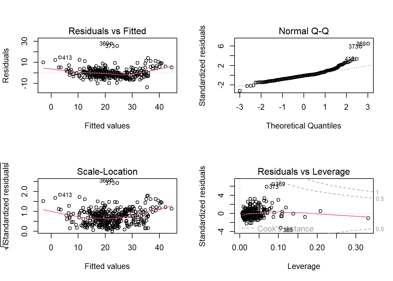
Residuals vs. Fitted plot shows that the relationship between medv and predictors is not completely linear. Also, normal qq plot is skewed implying that residuals are not normally distributed. A different functional from may be required.
Models are compared based on adjusted r square, AIC, BIC criteria for in-sample performance and mean square prediction error (MSPE) for out-of-sample performance.
par(mfrow = c(1,1))
#In-sample performance
#MSE
model4.sum <- summary(model4)
(model4.sum$sigma) ^ 2
## [1] 20.20108model5.sum <- summary(model5)
(model5.sum$sigma) ^ 2## [1] 20.09662#R-squared
model4.sum$r.squared## [1] 0.7570198model5.sum$r.squared## [1] 0.7569516#Adjusted r square
model4.sum$adj.r.squared## [1] 0.7483657model5.sum$adj.r.squared## [1] 0.7496668#AIC
AIC(model4, model5)| df | AIC |
|---|---|
| 15 | 2.23e+03 |
| 13 | 2.23e+03 |
#BIC
BIC(model4, model5)| df | BIC |
|---|---|
| 15 | 2.29e+03 |
| 13 | 2.28e+03 |
Finally, we can check the Out-of-sample Prediction or test error (MSPE):
model4.pred.test <- predict(model4, newdata = test)
model4.mspe <- mean((model4.pred.test - test$medv) ^ 2)
model4.mspe
## [1] 31.02748model5.pred.test <- predict(model5, newdata = test)
model5.mspe <- mean((model5.pred.test - test$medv) ^ 2)
model5.mspe## [1] 31.0118118.11 Cross Validation
Please check how function ?cv.glm works.
We will just extract from this object created by cv.glm command - the raw cross-validation estimate of prediction error.
#install.packages("boot")
library(boot)
model1.glm = glm(medv ~ ., data = houses)
cv.glm(data = houses, glmfit = model1.glm, K = 5)$delta[2]
## [1] 23.31673model2.glm = glm(medv ~ . -indus -age, data = houses)
cv.glm(data = houses, glmfit = model2.glm, K = 5)$delta[2]## [1] 23.61677Based on AIC criteria and adjusted R square values, model 2 is slightly better than model 1. In-sample MSE is nearly the same for both models.
We need to check out-of-sample MSPE for both models. Based on out-of-sample prediction error, model 2 is slightly better than model 1. MSPE of model 1 is 20.7113 while that of model 2 is 20.6784. Based on cross validation also, model 2 performs better.
18.12 Printing the final regression table
18.12.1 The ‘jtools’ package
Here, finally we can print our regression table with all properties, estimated coefficient for our 5 linear regression models using ‘jtools’ package:
if (requireNamespace("huxtable")) {
  # Export all 5 regressions with "Model #" labels,
  # standardized coefficients, and robust standard errors
export_summs(model1, model2, model3, model4, model5, model.names = c("Model 1","Model 2","Model 3", "Model 4", "Model 5"), scale = TRUE, robust=TRUE, digits=2, statistics=c(N="nobs", R2="r.squared",AIC="AIC"))
}| Model 1 | Model 2 | Model 3 | Model 4 | Model 5 | |
|---|---|---|---|---|---|
| (Intercept) | 22.11 *** | 22.11 *** | 21.96 *** | 21.95 *** | 21.95 *** |
| (0.31) | (0.28) | (0.22) | (0.24) | (0.24) | |
| lstat | -6.66 *** | -15.55 *** | -10.63 *** | -3.18 ** | -3.21 *** |
| (0.42) | (1.16) | (2.02) | (0.98) | (0.80) | |
| `I(lstat^2)` | 9.28 *** | 6.86 *** | |||
| (1.07) | (1.29) | ||||
| crim | -1.27 *** | -0.94 ** | -0.94 ** | ||
| (0.26) | (0.33) | (0.32) | |||
| zn | 0.58 | 1.10 ** | 1.10 ** | ||
| (0.37) | (0.40) | (0.38) | |||
| indus | 0.29 | 0.09 | |||
| (0.34) | (0.36) | ||||
| chas | 2.21 | 2.37 | 2.38 | ||
| (1.52) | (1.56) | (1.56) | |||
| nox | -2.20 *** | -2.53 *** | -2.54 *** | ||
| (0.46) | (0.54) | (0.43) | |||
| rm | 2.25 ** | 2.61 ** | 2.59 *** | ||
| (0.74) | (0.80) | (0.73) | |||
| age | 0.62 | -0.10 | |||
| (0.63) | (0.60) | ||||
| dis | -2.41 *** | -3.10 *** | -3.09 *** | ||
| (0.47) | (0.55) | (0.57) | |||
| rad | 2.97 *** | 3.17 *** | 3.15 *** | ||
| (0.62) | (0.75) | (0.71) | |||
| tax | -2.41 *** | -2.67 *** | -2.62 *** | ||
| (0.48) | (0.54) | (0.58) | |||
| ptratio | -1.87 *** | -2.11 *** | -2.12 *** | ||
| (0.28) | (0.29) | (0.28) | |||
| black | 0.64 ** | 0.73 * | 0.72 * | ||
| (0.23) | (0.29) | (0.28) | |||
| N | 379 | 379 | 379 | 379 | 379 |
| R2 | 0.55 | 0.64 | 0.79 | 0.76 | 0.76 |
| AIC | 2438.59 | 2358.71 | 2172.14 | 2230.46 | 2226.57 |
| All continuous predictors are mean-centered and scaled by 1 standard deviation. Standard errors are heteroskedasticity robust. *** p < 0.001; ** p < 0.01; * p < 0.05. | |||||
18.12.2 The final model
For the multiple regression models we decided, that our model2.glm performs best - so here we can print that model together with its VIF coefficients:
if (requireNamespace("huxtable")) {
export_summs(model2.glm, model.names = c("Final version of the MRM"), statistics=c(N="nobs", R2="r.squared",AIC="AIC", BIC="BIC"), vifs= TRUE, scale = TRUE, robust=TRUE, digits=2)
}| Final version of the MRM | |
|---|---|
| (Intercept) | 22.34 *** |
| (0.22) | |
| crim | -0.93 *** |
| (0.28) | |
| zn | 1.07 *** |
| (0.32) | |
| chas | 2.72 ** |
| (0.85) | |
| nox | -2.01 *** |
| (0.41) | |
| rm | 2.67 *** |
| (0.29) | |
| dis | -3.14 *** |
| (0.39) | |
| rad | 2.61 *** |
| (0.55) | |
| tax | -1.99 *** |
| (0.57) | |
| ptratio | -2.05 *** |
| (0.28) | |
| black | 0.85 *** |
| (0.24) | |
| lstat | -3.73 *** |
| (0.34) | |
| N | 506 |
| AIC | 3023.73 |
| BIC | 3078.67 |
| All continuous predictors are mean-centered and scaled by 1 standard deviation. Standard errors are heteroskedasticity robust. *** p < 0.001; ** p < 0.01; * p < 0.05. | |
# note that if you will change export_summs command into summ the table will be generated here!18.12.3 The ‘stargazer’ package
We can also use the ‘stargazer’ package to generate more user-friendly tables together with RMSE’s.
For this version of report printing - you will need your own TEX driver - usually it is the MikTex driver for Windows machines or MacTex for Mac computers.
We use Tex reports for PDF Markdown reports only. So put [include=TRUE] when using it:
18.12.4 The “modelsummary” package
“modelsummary” includes a powerful set of utilities to customize the information displayed in your model summary tables. You can easily rename, reorder, subset or omit parameter estimates; choose the set of goodness-of-fit statistics to display; display various “robust” standard errors or confidence intervals; add titles, footnotes, or source notes; insert stars or custom characters to indicate levels of statistical significance; or add rows with supplemental information about your models.
library(modelsummary)
models <- list(model1,model2)
modelsummary(
  models,
  fmt = 2,
  estimate  = c("{estimate}{stars}",
                "{estimate} ({std.error})"
                ),
statistic = NULL)| Model 1 | Model 2 | |
|---|---|---|
| (Intercept) | 34.12*** | 41.79 (0.99) |
| lstat | −0.94*** | −2.20 (0.14) |
| I(lstat^2) | 0.04 (0.00) | |
| Num.Obs. | 379 | 379 |
| R2 | 0.552 | 0.639 |
| R2 Adj. | 0.551 | 0.637 |
| AIC | 2438.6 | 2358.7 |
| BIC | 2450.4 | 2374.5 |
| F | 463.971 | 332.497 |
| RMSE | 5.99 | 5.38 |
Please read more about all features of the “modelsummary” package here.