Chapter 19 GLM Regression
Generalized linear models are a class of regression model that generalize (duh) and extend classic linear regression. Generally the response variable in these models follows an exponential family distribution. The random component (Y) is related to the systematic component (Xs) through the link function. This allows us to model many different outcomes, including binary, count, and categorical.
Other than this brief description, I will not be covering the theory and statistics underlying these models. Instead, I would like to focus on the basics of running GLMs in R.
19.1 Maximum Likelihood
In the standard model setting we attempt to find parameters \(\theta\) that will maximize the probability of the data we actually observe. We’ll start with an observed random target vector \(y\) with \(i...N\) independent and identically distributed observations and some data-generating process underlying it \(f(\cdot|\theta)\). We are interested in estimating the model parameter(s), \(\theta\), that would make the data most likely to have occurred. The probability density function for \(y\) given some particular estimate for the parameters can be noted as \(f(y_i|\theta)\).
The joint probability distribution of the (independent) observations given those parameters, \(f(y_i|\theta)\), is the product of the individual densities, and is our likelihood function.
We can write it out generally as: \[\mathcal{L}(\theta) = \prod_{i=1}^N f(y_i|\theta)\] Thus, the likelihood for one set of parameter estimates given a fixed set of data y, is equal to the probability of the data given those (fixed) estimates.
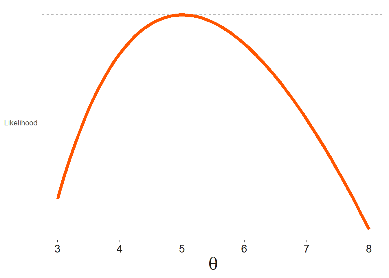
Furthermore, we can compare one set, \(\mathcal{L}(\theta_A)\), to that of another, \(\mathcal{L}(\theta_B)\), and whichever produces the greater likelihood would be the preferred set of estimates. We can get a sense of this with the following visualization, based on a single parameter.
The data is drawn from Poisson distributed variable with mean \(\theta=5\). We note the calculated likelihood increases as we estimate values for \(\theta\) closer to \(5\), or more precisely, whatever the mean observed value is for the data. However, with more and more data, the final ML estimate will converge on the true value.
For computational reasons, we instead work with the sum of the natural log probabilities, and so deal with the log likelihood:
\[\ln\mathcal{L}(\theta) = \sum_{i=1}^N \ln[f(y_i|\theta)]\]
Concretely, we calculate a log likelihood for each observation and then sum them for the total likelihood for parameter(s) \(\theta\).
The likelihood function incorporates our assumption about the sampling distribution of the data given some estimate for the parameters. It can take on many forms and be notably complex depending on the model in question, but once specified, we can use any number of optimization approaches to find the estimates of the parameter that make the data most likely. As an example, for a normally distributed variable of interest we can write the log likelihood as follows:
\[\ln\mathcal{L}(\theta) = \sum_{i=1}^N \ln[\frac{1}{\sqrt{2\pi\sigma^2}}\exp(-\frac{(y-\mu)^2}{2\sigma^2})]\]
19.2 Beyond linear models
What other kinds of models are there?
Linear regression models, as we’ve said, are useful and ubiquitous. But there’s a lot else out there. What else?
- Logistic regression
- Poisson regression
- Generalized linear models
- Generalized additive models
- Many, many others (generative models, Bayesian models, nonparametric models, machine learning “models”, etc.)
In this chapter we’ll quickly visit logit and probit models. In some ways, they are similar to linear regression; in others, they’re quite different.
19.3 Logistic regression
Probably the most common version of the GLM used is logistic regression. Typically, logistic regression is used to model binary outcomes, although it can essentially also model probabilities between 0 and 1, because its goal is to estimate parameters interpretable in terms of probabilities.
Logistic regression consists of:
The logistic or logit function refers to the link. The logistic (logit) function is \(1/(1+exp(-x))\), and it is the inverse of log-odds: \(log(p/(1-p))\).
A binomial error distribution is the distribution of expected heads you’d get when flipping a biased coin N times. Thus, it is appropriate for any two-level distribution in which you can represent the values as 0 and 1.
Given response \(Y\) and predictors \(X_1,\ldots,X_p\), where \(Y \in \{0,1\}\) is a binary outcome. In a logistic regression model, we posit the relationship:
\[ \log\frac{\mathbb{P}(Y=1|X)}{\mathbb{P}(Y=0|X)} = \beta_0 + \beta_1 X_1 + \ldots + \beta_p X_p \]
(where \(Y|X\) is shorthand for \(Y|X_1,\ldots,X_p\)). Goal is to estimate parameters, also called coefficients \(\beta_0,\beta_1,\ldots,\beta_p\)
19.3.1 Fitting a logistic regression model with glm()
We can use glm() to fit a logistic regression model. The arguments are very similar to lm()
The first argument is a formula, of the form Y ~ X1 + X2 + ... + Xp, where Y is the response and X1, …, Xp are the predictors. These refer to column names of variables in a data frame, that we pass in through the data argument. We must also specify family="binomial" to get logistic regression
What does a logistic regression coefficient mean?
How do you interpret a logistic regression coefficient? Note, from our logistic model:
\[ \frac{\mathbb{P}(Y=1|X)}{\mathbb{P}(Y=0|X)} = \exp(\beta_0 + \beta_1 X_1 + \ldots + \beta_p X_p) \]
So, increasing predictor \(X_j\) by one unit, while holding all other predictor fixed, multiplies the odds by \(e^{\beta_j}\).
19.3.2 Log-odds transform
Binary outcomes can be modeled with standard regression, but they are difficult to interpret. For example, we can model the the outcome of 0 or 1, but the predicted value won’t be all 0s or 1s, and typically won’t even be bounded between 0 and 1. To make a classification, we would need to come up with some (possibly ad-hoc) rule and state that any value above 0.5 should be called a 1. If we wanted to model probabilities instead of just 0/1 values, we arrive at a similar problem – there is no guarantee that the model will produce estimates bounded within [0,1]. This is disturbing, because you could have a reasonably good model that predicts your chance of something happenning is less than 0, or greater than 1.
One way to deal with this is to model the odds, which is \(p/(1-p)\). Now, there is no upper bound–as we get close to p=1.0, odds approaches INF. Furthermore, probabilities less than 0.5 are not symmetric with probabliities above 0.5. A log transform of odds fixes both of these issues (see second figure).
library(ggplot2)
p <- 0:100/100
odds <- p/(1-p)
logodds <- log(odds)
df <- data.frame(p,odds,logodds)
ggplot(df,aes(x=p,y=odds))+geom_line() + ggtitle("p versus odds(p)")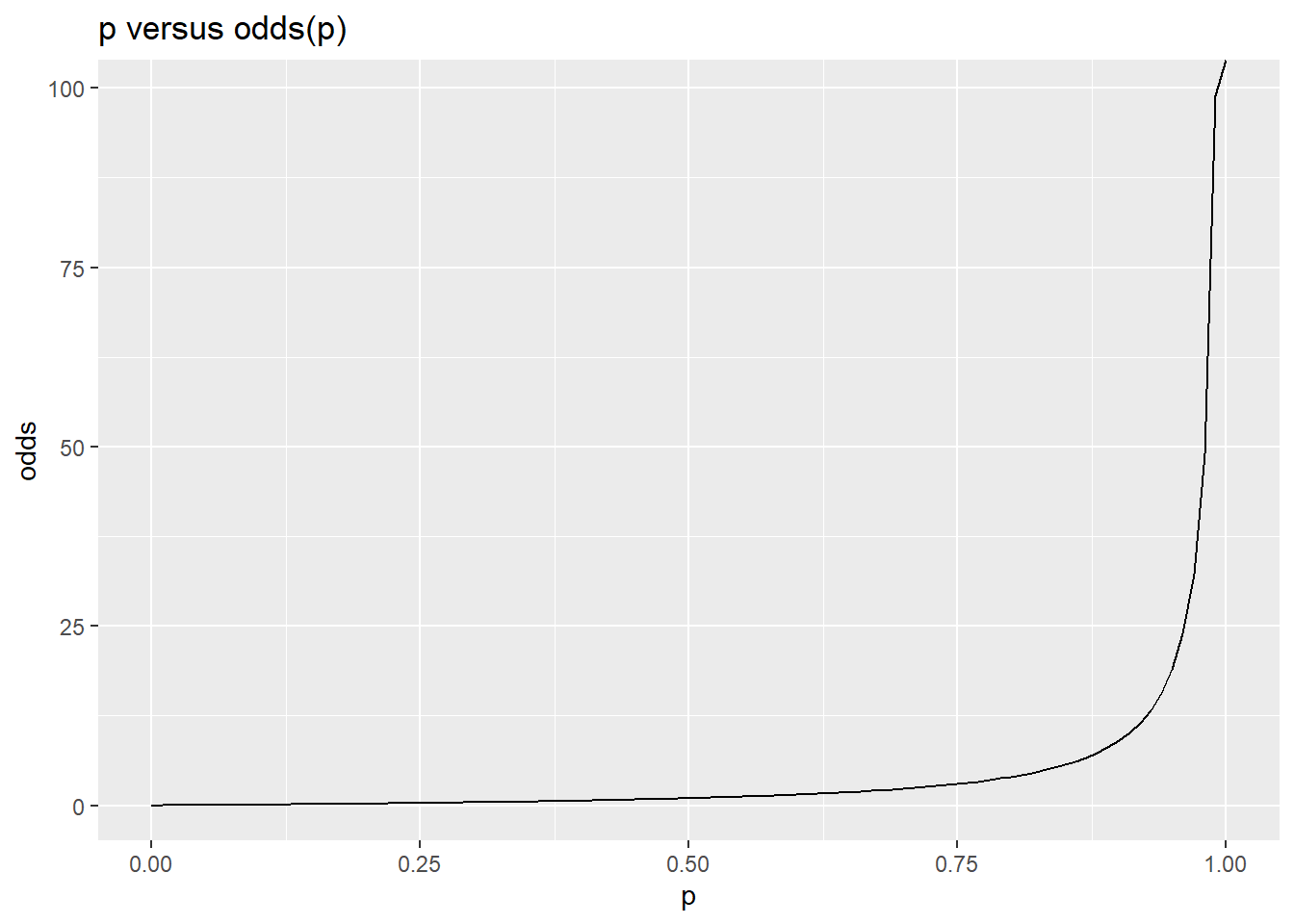
ggplot(df,aes(x=p,y=logodds))+geom_line() + ggtitle("p versus logodds(p)")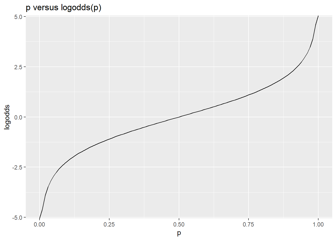
This gives a way of modeling a family of relationships between a continuous predictor and a binary outcome variable, by assuming that a predictor is linearly related to the log-odds (and then using this transform to convert to probability, and compute likelihood of data). By fitting the equivalent of an intercept term, we move this curve left and right. By fitting slopes with respect to a predictor, we make the curve sharper or flatter. The logistic is always symmetric around .5, and must start at 0 and go to 1.0, but otherwise is very flexible in modeling all kinds binary, probability, and two-level categorical variables.
ggplot(df,aes(x=logodds,y=p))+geom_line() + ggtitle("logodds(p) versus p")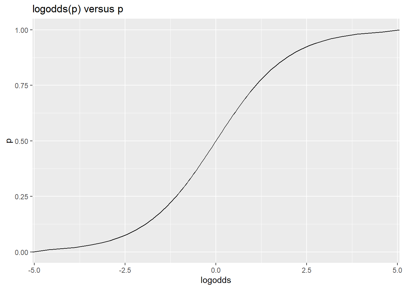
So, logistic regression transforms the outcomes so that a linear combination of predictors produces log-odds effects on the outcome. Any coefficient of the model can be transformed and interpreted as odds multiplier. This is the source of many news reports suggesting things like “smoking increases the odds of dying of cancer by X”. These results are easily interpretable by the public, and come directly from logistic regression models.
19.3.3 Worked Example
The birthwt data set has 130 children with a birthweight above 2.5 kilos, and 59 below, and many potential predictors. In regular regression, we might consider modeling the continuous weight value, but instead, we might want to model low birth weight, which could indicate risk. This is binary, and so is appropriate for a logistic regression. Let’s model this and see how a number of risk factors to at predicting low birth weight.
The following code estimates a logistic regression model using the glm (generalized linear model) function. Specifying the “family” of the model allows us to get the right distribution.
library(MASS)  #for birthwt data:
data(birthwt)

summary(birthwt)
## low age lwt race
## Min. :0.0000 Min. :14.00 Min. : 80.0 Min. :1.000
## 1st Qu.:0.0000 1st Qu.:19.00 1st Qu.:110.0 1st Qu.:1.000
## Median :0.0000 Median :23.00 Median :121.0 Median :1.000
## Mean :0.3122 Mean :23.24 Mean :129.8 Mean :1.847
## 3rd Qu.:1.0000 3rd Qu.:26.00 3rd Qu.:140.0 3rd Qu.:3.000
## Max. :1.0000 Max. :45.00 Max. :250.0 Max. :3.000
## smoke ptl ht ui
## Min. :0.0000 Min. :0.0000 Min. :0.00000 Min. :0.0000
## 1st Qu.:0.0000 1st Qu.:0.0000 1st Qu.:0.00000 1st Qu.:0.0000
## Median :0.0000 Median :0.0000 Median :0.00000 Median :0.0000
## Mean :0.3915 Mean :0.1958 Mean :0.06349 Mean :0.1481
## 3rd Qu.:1.0000 3rd Qu.:0.0000 3rd Qu.:0.00000 3rd Qu.:0.0000
## Max. :1.0000 Max. :3.0000 Max. :1.00000 Max. :1.0000
## ftv bwt
## Min. :0.0000 Min. : 709
## 1st Qu.:0.0000 1st Qu.:2414
## Median :0.0000 Median :2977
## Mean :0.7937 Mean :2945
## 3rd Qu.:1.0000 3rd Qu.:3487
## Max. :6.0000 Max. :4990table(birthwt$low)##
## 0 1
## 130 59Note: we are leaving off the variable bwt. (This would allow us to predict perfectly.)
Build the model. Note that we don’t transform the outcome – we let the default ‘logit’ link function of the binomial family regression handle that for us.
full.model <- glm(low~age+lwt+factor(race)+smoke+ptl+ht+ui+ftv,
                  data=birthwt,family=binomial())
summary(full.model)
##
## Call:
## glm(formula = low ~ age + lwt + factor(race) + smoke + ptl +
## ht + ui + ftv, family = binomial(), data = birthwt)
##
## Deviance Residuals:
## Min 1Q Median 3Q Max
## -1.8946 -0.8212 -0.5316 0.9818 2.2125
##
## Coefficients:
## Estimate Std. Error z value Pr(>|z|)
## (Intercept) 0.480623 1.196888 0.402 0.68801
## age -0.029549 0.037031 -0.798 0.42489
## lwt -0.015424 0.006919 -2.229 0.02580 *
## factor(race)2 1.272260 0.527357 2.413 0.01584 *
## factor(race)3 0.880496 0.440778 1.998 0.04576 *
## smoke 0.938846 0.402147 2.335 0.01957 *
## ptl 0.543337 0.345403 1.573 0.11571
## ht 1.863303 0.697533 2.671 0.00756 **
## ui 0.767648 0.459318 1.671 0.09467 .
## ftv 0.065302 0.172394 0.379 0.70484
## ---
## Signif. codes: 0 '***' 0.001 '**' 0.01 '*' 0.05 '.' 0.1 ' ' 1
##
## (Dispersion parameter for binomial family taken to be 1)
##
## Null deviance: 234.67 on 188 degrees of freedom
## Residual deviance: 201.28 on 179 degrees of freedom
## AIC: 221.28
##
## Number of Fisher Scoring iterations: 4The model seems reasonable, with many of the predictors significant. Looking at the significant predictors we see last mother’s weight, race, smoking, history of hypertension are significant predictors. Weight is negative, which means that the less a mother weighs, the greater the risk of low birth weight. The others are all positive.
The coefficients close to 0 have no impact on log-odds, whereas values above 0 have a positive impact, and values below 0 a negative impact – keep in mind that log-odds(.5)=0.
Interpreting the results output: * the first row reminds us what function we called * deviance residuals is a measure of model fit * The next table shows coeeficients, std error, z statistic - all the factors are statistically significant (last column), for every one unit change in hypertensiom (ht) the odds of low bithweight increases by 1.749
19.3.4 Over-dispersion
The Logistic model assumes errors happen exactly like tossing a single coin multiple times. The coin may be biased, but we assume it is the same biased coin. But what would happen if the data were really like a jar of coins, each with a different bias? For each observation, we pick a coin and then flip it. It turns out that this would create different error distributions, and lead us to make incorrect inference. This is called over-dispersion, and it should be checked for in a logistic regression. In logistic regression, unlike in OLS, the binomial error distribution makes a strong assumption about the relationship between p and sd(p)==it should be \(\sqrt{(p*(1-p))}\). If it is not, we have an additional source of noise in the sampling.
Returning to the birth weight data, We should check for over-dispersion. If the logistic assumptions hold, residual deviance should be about the same as the degrees of freedom. If much larger, this indicates over-dispersion, and could mean we have dependencies among our data, such as you’d find in repeated-measures experiments, or variability in the sampling of people like the coin-sampling. If you are modeling accuracy in a study, and accuracy differs systematically across people, but model mean accuracy in a logistic regression, you are likely to find over-dispersion.
Let’s look at a smaller model tha involves just the significant factors:
partial.model <- glm(low~lwt+factor(race)+smoke+ht,data=birthwt,family=binomial())
summary(partial.model)
##
## Call:
## glm(formula = low ~ lwt + factor(race) + smoke + ht, family = binomial(),
## data = birthwt)
##
## Deviance Residuals:
## Min 1Q Median 3Q Max
## -1.7751 -0.8747 -0.5712 0.9634 2.1131
##
## Coefficients:
## Estimate Std. Error z value Pr(>|z|)
## (Intercept) 0.352049 0.924438 0.381 0.70333
## lwt -0.017907 0.006799 -2.634 0.00844 **
## factor(race)2 1.287662 0.521648 2.468 0.01357 *
## factor(race)3 0.943645 0.423382 2.229 0.02583 *
## smoke 1.071566 0.387517 2.765 0.00569 **
## ht 1.749163 0.690820 2.532 0.01134 *
## ---
## Signif. codes: 0 '***' 0.001 '**' 0.01 '*' 0.05 '.' 0.1 ' ' 1
##
## (Dispersion parameter for binomial family taken to be 1)
##
## Null deviance: 234.67 on 188 degrees of freedom
## Residual deviance: 208.25 on 183 degrees of freedom
## AIC: 220.25
##
## Number of Fisher Scoring iterations: 4That looks pretty good. The predictors are significant (last column). The residual deviance is a bit larger than the degrees of freedom–maybe by about 10%. But this lack of fit could come from many sources–including violations of all the same assumptions of linear regression, such as non-normal predictors, non-linearity in the predictors, etc. If we examine the only continuous predict lwt, we see some skew that might deserve a transformation, but checking this it does not impact residual variance.
A 10% higher than expected deviance is probably not unexpected, and would be fairly common to see if there was no over-dispersion (this can be tested with a chi squared test). And because the data are all binary (0/1), it would be difficult to find overdispersion. But logistic models can be used for proportions and probabilities too, and a we will see below, these can be overdispersed.
If you have large overdispersion, you may need to use a package like ‘dispmod’, which can handle a binomial overdispersed logit model. However, the package does not seem to work on this model. It will work on the example in the help, in which each case is a number of successes out several different numbers of seeds. The issue is that there are two ways of specifying the dvs of a glm logistic, either as 0/1 (which we have here), or if you have more than 1 observation per grouping, as a two column matrix with \(x\) and \((n-x)\). The dispmod wants the second kind, but the second kind won’t work with just 1 observation per line. But with just one observation per case, you are likely to match the assumptions of the binomial model and so overdispersion would not be a problem. To fake this, let’s just assume we have 2 observations per group, by multiplying everything by 2. We would not do this if we really wanted to use dispmod to estimate overdispersion for our data–we are just doing it to see what the results would have been if that were the case.
library(dispmod)
dv <- cbind(birthwt$low,1-birthwt$low)*2
partial.model <- glm(dv~lwt+age,data=birthwt,family=binomial(logit))
model.od2 <- glm.binomial.disp(partial.model,verbose=T)
##
## Binomial overdispersed logit model fitting...
## Iter. 1 phi: 1.036053
## Converged after 1 iterations.
## Estimated dispersion parameter: 1.036053
##
## Call:
## glm(formula = dv ~ lwt + age, family = binomial(logit), data = birthwt,
## weights = disp.weights)
##
## Deviance Residuals:
## Min 1Q Median 3Q Max
## -1.1251 -0.9007 -0.7413 1.3273 2.0412
##
## Coefficients:
## Estimate Std. Error z value Pr(>|z|)
## (Intercept) 1.748773 1.006012 1.738 0.0822 .
## lwt -0.012775 0.006267 -2.039 0.0415 *
## age -0.039788 0.032576 -1.221 0.2219
## ---
## Signif. codes: 0 '***' 0.001 '**' 0.01 '*' 0.05 '.' 0.1 ' ' 1
##
## (Dispersion parameter for binomial family taken to be 1)
##
## Null deviance: 230.52 on 188 degrees of freedom
## Residual deviance: 223.10 on 186 degrees of freedom
## AIC: 229.1
##
## Number of Fisher Scoring iterations: 4model.od2##
## Call: glm(formula = dv ~ lwt + age, family = binomial(logit), data = birthwt,
## weights = disp.weights)
##
## Coefficients:
## (Intercept) lwt age
## 1.74877 -0.01278 -0.03979
##
## Degrees of Freedom: 188 Total (i.e. Null); 186 Residual
## Null Deviance: 230.5
## Residual Deviance: 223.1 AIC: 229.1print(paste("Dispersion parameter is:",model.od2$dispersion))## [1] "Dispersion parameter is: 1.03605253501365"The typical solution is to use the quasibinomial family, which also estimates a dispersion parameter for you.
partial.model2 <- glm(low ~ lwt + factor(race) + smoke + ht, data=birthwt,family=quasibinomial(logit))

summary(partial.model2)
##
## Call:
## glm(formula = low ~ lwt + factor(race) + smoke + ht, family = quasibinomial(logit),
## data = birthwt)
##
## Deviance Residuals:
## Min 1Q Median 3Q Max
## -1.7751 -0.8747 -0.5712 0.9634 2.1131
##
## Coefficients:
## Estimate Std. Error t value Pr(>|t|)
## (Intercept) 0.352049 0.928263 0.379 0.70494
## lwt -0.017907 0.006827 -2.623 0.00945 **
## factor(race)2 1.287662 0.523806 2.458 0.01489 *
## factor(race)3 0.943645 0.425133 2.220 0.02767 *
## smoke 1.071566 0.389120 2.754 0.00648 **
## ht 1.749163 0.693678 2.522 0.01254 *
## ---
## Signif. codes: 0 '***' 0.001 '**' 0.01 '*' 0.05 '.' 0.1 ' ' 1
##
## (Dispersion parameter for quasibinomial family taken to be 1.008291)
##
## Null deviance: 234.67 on 188 degrees of freedom
## Residual deviance: 208.25 on 183 degrees of freedom
## AIC: NA
##
## Number of Fisher Scoring iterations: 4Here, the estimate is very close to 1.0, indicating no overdispersion, which is akin to the dispmod approach.
19.3.5 Comparing overall models
Now, to find out if the overall regression is significant (not just the individual predictors) we must compare two models. We need to specify the test to use, and usually one uses a chi-squared test to compare logistic models:
full.model <- glm(low~age+lwt+factor(race)+smoke+ptl+ht+ui+ftv,
                  data=birthwt,family=binomial())

partial.model <- glm(low~age+lwt+factor(race),
                  data=birthwt,family=binomial())

anova(partial.model, full.model, test="Chisq")
## Analysis of Deviance Table
##
## Model 1: low ~ age + lwt + factor(race)
## Model 2: low ~ age + lwt + factor(race) + smoke + ptl + ht + ui + ftv
## Resid. Df Resid. Dev Df Deviance Pr(>Chi)
## 1 184 222.66
## 2 179 201.28 5 21.376 0.0006877 ***
## ---
## Signif. codes: 0 '***' 0.001 '**' 0.01 '*' 0.05 '.' 0.1 ' ' 1The result suggests that the partial model is adequate for predicting low birth weight. Chi-Squared is not significant, so we would prefer the smaller model.
An alternative is doing a wald-test, which is available in the lmtest and aod packages. The wald test is essentially a t-test for individual coefficients, but we know that a t-test on linear regression coefficients is equivalent to the F-test on nested models.
library(lmtest)
waldtest(partial.model)
## Wald test
##
## Model 1: low ~ age + lwt + factor(race)
## Model 2: low ~ 1
## Res.Df Df F Pr(>F)
## 1 184
## 2 188 -4 2.6572 0.03436 *
## ---
## Signif. codes: 0 '***' 0.001 '**' 0.01 '*' 0.05 '.' 0.1 ' ' 1waldtest(full.model) ## Wald test
##
## Model 1: low ~ age + lwt + factor(race) + smoke + ptl + ht + ui + ftv
## Model 2: low ~ 1
## Res.Df Df F Pr(>F)
## 1 179
## 2 188 -9 2.856 0.003603 **
## ---
## Signif. codes: 0 '***' 0.001 '**' 0.01 '*' 0.05 '.' 0.1 ' ' 1waldtest(full.model,"lwt")## Wald test
##
## Model 1: low ~ age + lwt + factor(race) + smoke + ptl + ht + ui + ftv
## Model 2: low ~ age + factor(race) + smoke + ptl + ht + ui + ftv
## Res.Df Df F Pr(>F)
## 1 179
## 2 180 -1 4.9693 0.02705 *
## ---
## Signif. codes: 0 '***' 0.001 '**' 0.01 '*' 0.05 '.' 0.1 ' ' 1waldtest(full.model,"lwt",test="Chisq")## Wald test
##
## Model 1: low ~ age + lwt + factor(race) + smoke + ptl + ht + ui + ftv
## Model 2: low ~ age + factor(race) + smoke + ptl + ht + ui + ftv
## Res.Df Df Chisq Pr(>Chisq)
## 1 179
## 2 180 -1 4.9693 0.0258 *
## ---
## Signif. codes: 0 '***' 0.001 '**' 0.01 '*' 0.05 '.' 0.1 ' ' 1Notice that we can do the same comparisons using \(\chi^2\) tests using either ANOVA or wald, but they produce different results. I haven’t found any clear discussion of how these differ or if one is preferred.
anova(partial.model, full.model, test="Chisq")## Analysis of Deviance Table
##
## Model 1: low ~ age + lwt + factor(race)
## Model 2: low ~ age + lwt + factor(race) + smoke + ptl + ht + ui + ftv
## Resid. Df Resid. Dev Df Deviance Pr(>Chi)
## 1 184 222.66
## 2 179 201.28 5 21.376 0.0006877 ***
## ---
## Signif. codes: 0 '***' 0.001 '**' 0.01 '*' 0.05 '.' 0.1 ' ' 1waldtest(full.model,partial.model,test="Chisq")## Wald test
##
## Model 1: low ~ age + lwt + factor(race) + smoke + ptl + ht + ui + ftv
## Model 2: low ~ age + lwt + factor(race)
## Res.Df Df Chisq Pr(>Chisq)
## 1 179
## 2 184 -5 18.922 0.001988 **
## ---
## Signif. codes: 0 '***' 0.001 '**' 0.01 '*' 0.05 '.' 0.1 ' ' 119.4 Modeling probabilities
Here, I will create some random data from a group of participants (each of 10 participants \(obs\) produced 100 trials).
The outcome is randomly selected to be 0/1 based on the a ‘predictor’ which you might interpret as condition – the higher the condition number, the greater the probability of success.
But different subjects are different – some have low accuracy and others have higher accuracy.
obs <- rep(1:10,each=100)
predictor <- rep(1:10,100)
subadd <- rnorm(10)
outcome <- (predictor + rnorm(1000)*2 +subadd[obs]) >.5

plot(aggregate(outcome,list(predictor), mean),main="Overall accuracy")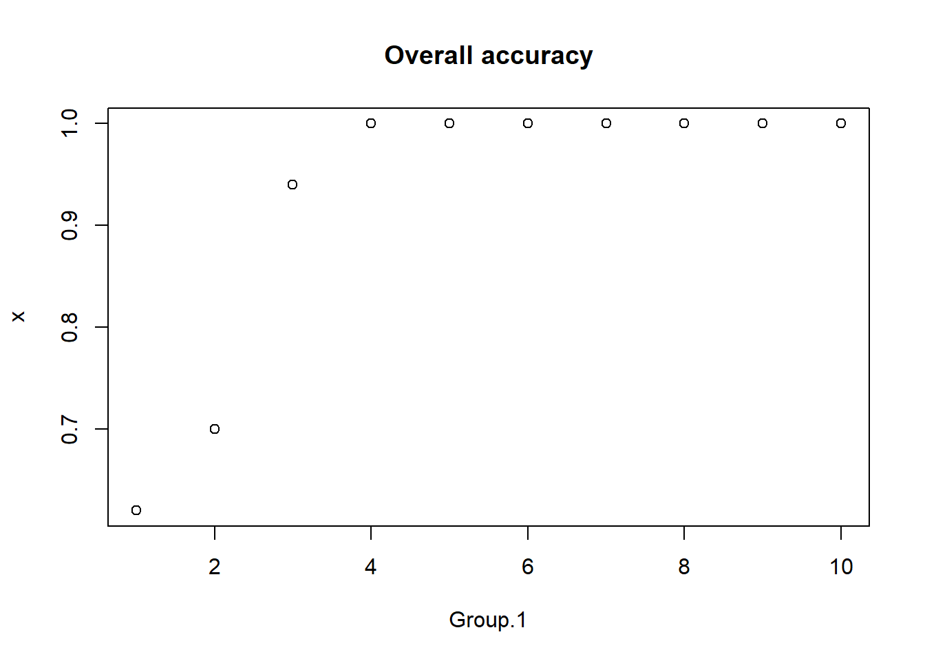
matplot(tapply(outcome,list(predictor,obs),mean),type="l",col="black",lty=1,ylab="Accuracy",main="Accuracy by participant")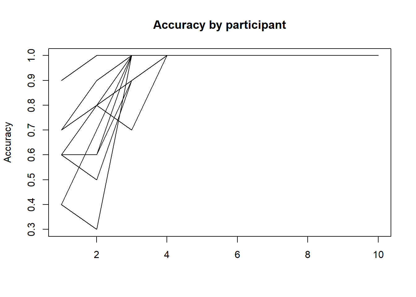
Let’s aggregate the data in two ways: first by just taking the sum of successes/total cases, and second by calculating the mean accuracy.
data.agg <- aggregate(outcome,list(predictor=predictor,obs=obs),sum)
data.agg$n <- aggregate(outcome,list(predictor),length)$x
data.agg$sub <- as.factor(data.agg$obs)
data.agg2 <-  aggregate(outcome,list(predictor=predictor,obs=as.factor(obs)),mean)
We can fit a logistic model either to the two column matrix of x and (n-x) in (number of successes out of total), or on the probability values in agg2. In both cases, we have underdispersion because participant noise existed.
m3a <- glm(cbind(x,n-x) ~ predictor, data=data.agg, family=binomial(logit))
m3b <- glm(cbind(x,n-x) ~ predictor, data=data.agg, family=quasibinomial(logit))
summary(m3a)
##
## Call:
## glm(formula = cbind(x, n - x) ~ predictor, family = binomial(logit),
## data = data.agg)
##
## Deviance Residuals:
## Min 1Q Median 3Q Max
## -2.10953 -0.19829 0.08333 0.33121 0.69273
##
## Coefficients:
## Estimate Std. Error z value Pr(>|z|)
## (Intercept) -2.51975 0.07781 -32.38 < 2e-16 ***
## predictor 0.04209 0.01206 3.49 0.000482 ***
## ---
## Signif. codes: 0 '***' 0.001 '**' 0.01 '*' 0.05 '.' 0.1 ' ' 1
##
## (Dispersion parameter for binomial family taken to be 1)
##
## Null deviance: 34.341 on 99 degrees of freedom
## Residual deviance: 22.108 on 98 degrees of freedom
## AIC: 422.56
##
## Number of Fisher Scoring iterations: 4summary(m3b)##
## Call:
## glm(formula = cbind(x, n - x) ~ predictor, family = quasibinomial(logit),
## data = data.agg)
##
## Deviance Residuals:
## Min 1Q Median 3Q Max
## -2.10953 -0.19829 0.08333 0.33121 0.69273
##
## Coefficients:
## Estimate Std. Error t value Pr(>|t|)
## (Intercept) -2.519749 0.035282 -71.417 < 2e-16 ***
## predictor 0.042092 0.005468 7.697 1.12e-11 ***
## ---
## Signif. codes: 0 '***' 0.001 '**' 0.01 '*' 0.05 '.' 0.1 ' ' 1
##
## (Dispersion parameter for quasibinomial family taken to be 0.2056244)
##
## Null deviance: 34.341 on 99 degrees of freedom
## Residual deviance: 22.108 on 98 degrees of freedom
## AIC: NA
##
## Number of Fisher Scoring iterations: 4Now, we can detect the under-dispersion stemming from within-subject correlation, as the dispersion parameter ends up being .32. The systematic individual differences produce less randomness than we would expect from the binomial model which assumes all people are the same.
If instead, we use agg2, for which we already calculated the probabilities within each subject, we can fit the same models:
m4a <- glm(x ~ predictor, data=data.agg2,family=binomial)
m4b <- glm(x ~ predictor, data=data.agg2,family=quasibinomial)
summary(m4a)
##
## Call:
## glm(formula = x ~ predictor, family = binomial, data = data.agg2)
##
## Deviance Residuals:
## Min 1Q Median 3Q Max
## -1.09776 0.00913 0.03146 0.10825 0.77073
##
## Coefficients:
## Estimate Std. Error z value Pr(>|z|)
## (Intercept) -1.0483 0.9369 -1.119 0.26320
## predictor 1.2370 0.4677 2.645 0.00817 **
## ---
## Signif. codes: 0 '***' 0.001 '**' 0.01 '*' 0.05 '.' 0.1 ' ' 1
##
## (Dispersion parameter for binomial family taken to be 1)
##
## Null deviance: 27.0349 on 99 degrees of freedom
## Residual deviance: 5.7327 on 98 degrees of freedom
## AIC: 28.744
##
## Number of Fisher Scoring iterations: 8summary(m4b)##
## Call:
## glm(formula = x ~ predictor, family = quasibinomial, data = data.agg2)
##
## Deviance Residuals:
## Min 1Q Median 3Q Max
## -1.09776 0.00913 0.03146 0.10825 0.77073
##
## Coefficients:
## Estimate Std. Error t value Pr(>|t|)
## (Intercept) -1.0483 0.2285 -4.588 1.33e-05 ***
## predictor 1.2370 0.1141 10.845 < 2e-16 ***
## ---
## Signif. codes: 0 '***' 0.001 '**' 0.01 '*' 0.05 '.' 0.1 ' ' 1
##
## (Dispersion parameter for quasibinomial family taken to be 0.05947667)
##
## Null deviance: 27.0349 on 99 degrees of freedom
## Residual deviance: 5.7327 on 98 degrees of freedom
## AIC: NA
##
## Number of Fisher Scoring iterations: 8Even though the model complains (non-integer successes), it will fit the data. The coefficients are different, and we would have to be careful trying to predict values. We can look at the predicted versus actual values (transforming with the logit function)
logit <- function(lo) {1/(1+exp(-lo))}
plot(data.agg2$x,logit(predict(m4b)),xlab="Mean accuracy",ylab="Predicted accuracy")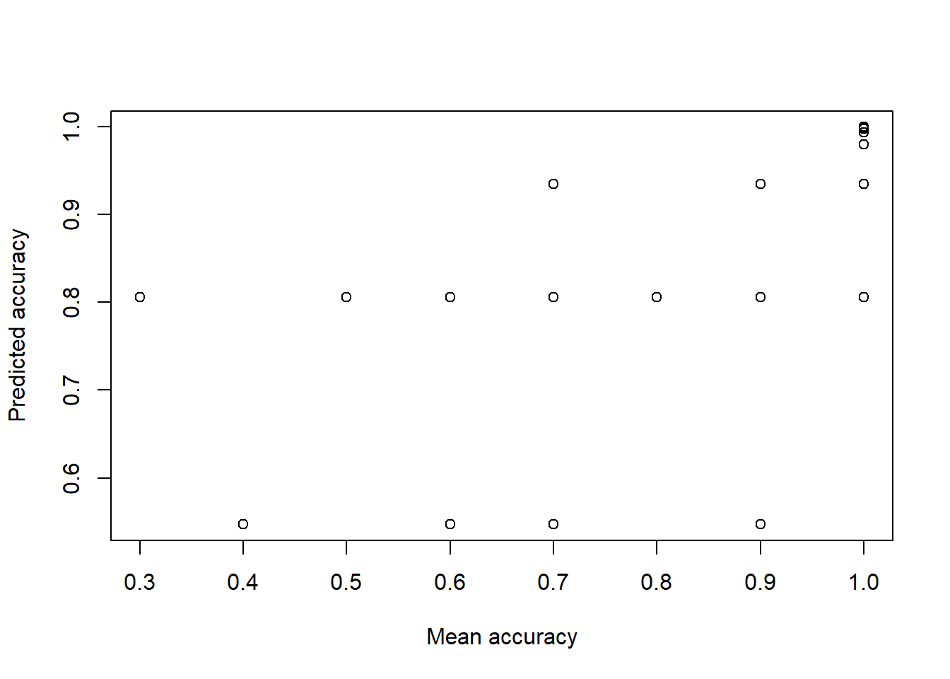
19.4.1 Dissecting the logistic model
Lets take a look at the probability mechanism underlying this function.
logodds <- function(p) {log(p/1-p)} ##The probability of a "yes" for a given set of predictor values.
logit <- function(lo) {1/(1+exp(-lo))} ##This is the inverse of the logodds function. The logistic function will
## map any value of the right hand side (z) to a proportion value between 0 and 1 (Manning, 2007)
19.4.2 Predicting
We can use Intercept +/- mother’s weight + smoking to make simple predictions about different aspects. Here are two groups that differ by the smoking coefficient, modeling the impact of mother’s weight on low birth weight.
plot(00:250, logit(.4806 + -.0154 * 0:250),ylim=c(0,1),xlab="Mother's weight",ylab="Probability low birth weight")
points(0:250,logit(.4806 + .9388 + -.0154 * 0:250),type="l",col="red")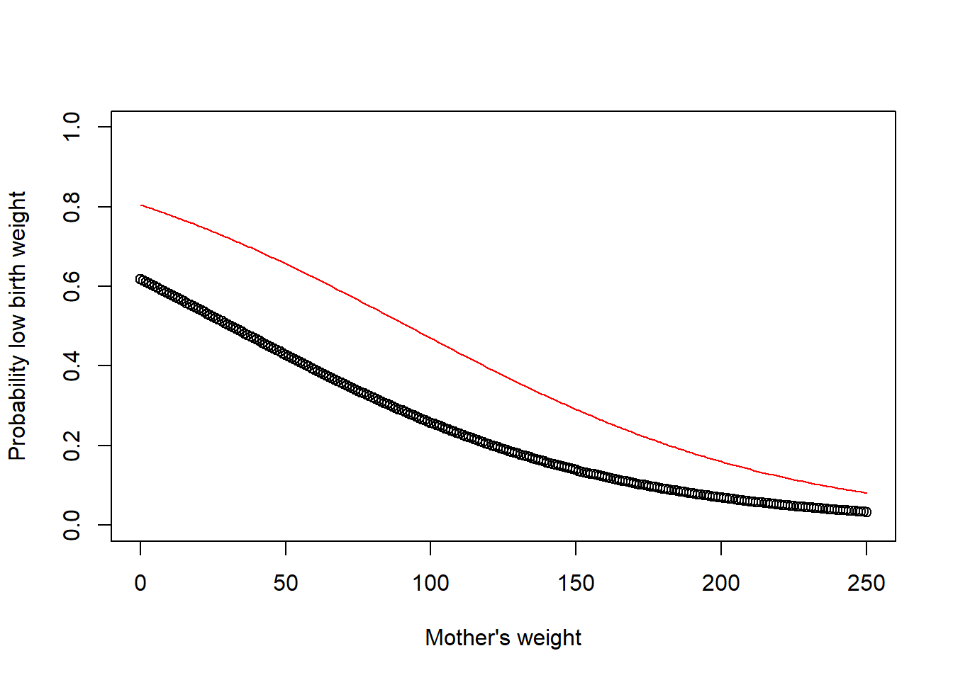 Notice that the impact of smoking is not constant over birth weight, but it is constant in log-odds terms, meaning the impact of smoking decreases as the overall probability gets closer to 0 or 1.
When we use the ‘predict’ function we can see the probability of a low birth weight baby based on the predictor variables we have chosen. If you look at the birthwt data set it’s interesting to compare the smoking variable with the overall prediction.
We can think about this another way:
coef(partial.model) ## (Intercept) age lwt factor(race)2 factor(race)3
## 1.30674122 -0.02552379 -0.01435323 1.00382195 0.44346082This gives us the change in (log)odds in response to a unit change in the predictor variable if all the other variables are held constant. It can be easier to interpret if the results are exponentiated to put the results in an odds scale.
exp(coef(partial.model))## Now we can see that the chances of having a low birth weight baby increase by a factor of## (Intercept) age lwt factor(race)2 factor(race)3
## 3.6941158 0.9747992 0.9857493 2.7286908 1.5580902## 5.75 if the mother has a history of hypertension and by 2.92 if the mother smokes during pregnancy.
exp(confint(partial.model))## 2.5 % 97.5 %
## (Intercept) 0.4752664 32.099365
## age 0.9117071 1.039359
## lwt 0.9724784 0.997786
## factor(race)2 1.0226789 7.322799
## factor(race)3 0.7679486 3.167985## gives us the 95 percent confidence interval for each of the coefficients on the odds scale. if it includes one we don't know if it has a difference. Greater than 1. 19.5 Case study
Example: Personality predicts smartphone choice
Recently, a study was published that establishes that personality factors can predict whether users report using an iphone or android device:
Quoting the abstract, “In comparison to Android users, we found that iPhone owners are more likely to be female, younger, and increasingly concerned about their smartphone being viewed as a status object. Key differences in personality were also observed with iPhone users displaying lower levels of Honesty Humility and higher levels of emotionality.”
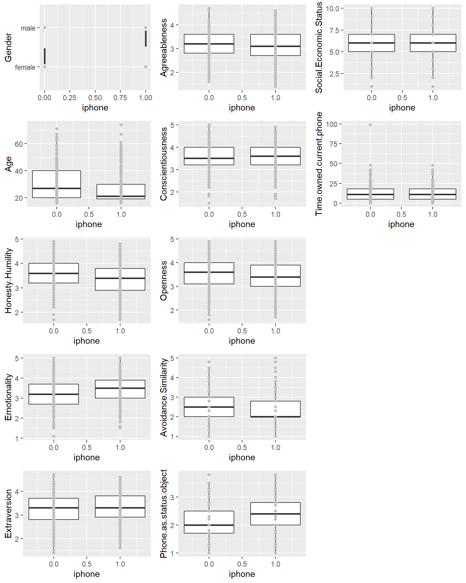
Let’s look at the data and see if we agree.
phone0 <- read.csv("data_study1.csv")
phone0$iphone <- (phone0$Smartphone=="iPhone")+0
phone <- phone0[,-1]
library(grid)

layout <- matrix(1:15,nrow=5,ncol=3)
  grid.newpage()
   pushViewport(viewport(layout = grid.layout(nrow(layout), ncol(layout))))

for(i in 1:12)
{
  var <- colnames(phone)[i]
    matchidx <- as.data.frame(which(layout == i, arr.ind = TRUE))
    x <-  ggplot(phone,aes_string(x="iphone",y=var)) +
      geom_boxplot(aes(group=iphone)) + geom_point(col="grey")
      print(x, vp = viewport(layout.pos.row = matchidx$row,
                          layout.pos.col = matchidx$col))
}
phone2 <- phone
phone2$Gender <- as.numeric(phone2$Gender)
table(phone$iphone)
##
## 0 1
## 219 310round(cor(as.matrix(phone2)),3)## Gender Age Honesty.Humility Emotionality
## Gender 1 NA NA NA
## Age NA 1.000 0.264 -0.222
## Honesty.Humility NA 0.264 1.000 0.040
## Emotionality NA -0.222 0.040 1.000
## Extraversion NA 0.113 0.036 -0.147
## Agreeableness NA 0.046 0.337 0.014
## Conscientiousness NA 0.081 0.289 0.088
## Openness NA 0.166 0.060 -0.146
## Avoidance.Similarity NA 0.092 0.027 -0.140
## Phone.as.status.object NA -0.247 -0.424 0.172
## Social.Economic.Status NA 0.067 0.015 -0.079
## Time.owned.current.phone NA 0.082 0.063 -0.087
## iphone NA -0.174 -0.194 0.159
## Extraversion Agreeableness Conscientiousness Openness
## Gender NA NA NA NA
## Age 0.113 0.046 0.081 0.166
## Honesty.Humility 0.036 0.337 0.289 0.060
## Emotionality -0.147 0.014 0.088 -0.146
## Extraversion 1.000 0.090 0.054 0.162
## Agreeableness 0.090 1.000 0.102 0.144
## Conscientiousness 0.054 0.102 1.000 0.076
## Openness 0.162 0.144 0.076 1.000
## Avoidance.Similarity 0.014 -0.111 -0.003 0.065
## Phone.as.status.object 0.054 -0.128 -0.160 -0.236
## Social.Economic.Status 0.303 -0.054 0.195 0.001
## Time.owned.current.phone 0.072 0.032 -0.007 0.094
## iphone 0.069 -0.042 0.024 -0.100
## Avoidance.Similarity Phone.as.status.object
## Gender NA NA
## Age 0.092 -0.247
## Honesty.Humility 0.027 -0.424
## Emotionality -0.140 0.172
## Extraversion 0.014 0.054
## Agreeableness -0.111 -0.128
## Conscientiousness -0.003 -0.160
## Openness 0.065 -0.236
## Avoidance.Similarity 1.000 -0.129
## Phone.as.status.object -0.129 1.000
## Social.Economic.Status -0.001 0.088
## Time.owned.current.phone -0.010 -0.178
## iphone -0.141 0.240
## Social.Economic.Status Time.owned.current.phone iphone
## Gender NA NA NA
## Age 0.067 0.082 -0.174
## Honesty.Humility 0.015 0.063 -0.194
## Emotionality -0.079 -0.087 0.159
## Extraversion 0.303 0.072 0.069
## Agreeableness -0.054 0.032 -0.042
## Conscientiousness 0.195 -0.007 0.024
## Openness 0.001 0.094 -0.100
## Avoidance.Similarity -0.001 -0.010 -0.141
## Phone.as.status.object 0.088 -0.178 0.240
## Social.Economic.Status 1.000 0.058 0.020
## Time.owned.current.phone 0.058 1.000 -0.051
## iphone 0.020 -0.051 1.000We see here that approximately 60% of respondents used the iphone – so we could be 60% correct just by claiming everyone chooses the iPhone. The correlations between phone choice and any individual personality trait or related question are all small–with the largest around .24. Because iPhone ownership can be categerized into two categories, a logistic regression model is appropriate:
model.full <- glm(iphone~.,data=phone,family=binomial())
summary(model.full)
##
## Call:
## glm(formula = iphone ~ ., family = binomial(), data = phone)
##
## Deviance Residuals:
## Min 1Q Median 3Q Max
## -2.2383 -1.0875 0.6497 0.9718 1.8392
##
## Coefficients:
## Estimate Std. Error z value Pr(>|z|)
## (Intercept) 3.158e-01 1.382e+00 0.228 0.81929
## Gendermale -6.356e-01 2.276e-01 -2.792 0.00523 **
## Age -1.429e-02 7.689e-03 -1.859 0.06305 .
## Honesty.Humility -5.467e-01 1.918e-01 -2.850 0.00437 **
## Emotionality 1.631e-01 1.626e-01 1.003 0.31598
## Extraversion 3.161e-01 1.603e-01 1.972 0.04859 *
## Agreeableness 4.070e-02 1.672e-01 0.243 0.80770
## Conscientiousness 2.802e-01 1.710e-01 1.639 0.10130
## Openness -1.441e-01 1.635e-01 -0.881 0.37827
## Avoidance.Similarity -2.653e-01 1.175e-01 -2.257 0.02399 *
## Phone.as.status.object 5.004e-01 1.931e-01 2.592 0.00955 **
## Social.Economic.Status -1.781e-02 6.741e-02 -0.264 0.79162
## Time.owned.current.phone 4.048e-06 9.608e-03 0.000 0.99966
## ---
## Signif. codes: 0 '***' 0.001 '**' 0.01 '*' 0.05 '.' 0.1 ' ' 1
##
## (Dispersion parameter for binomial family taken to be 1)
##
## Null deviance: 717.62 on 528 degrees of freedom
## Residual deviance: 644.17 on 516 degrees of freedom
## AIC: 670.17
##
## Number of Fisher Scoring iterations: 4Looking at the results, we can see that a handful of predictors are significant. Importantly, gender and phone-as-status-object are fairly strong, as well as avoidance of similarity.
Some things to note:
- Negative and positive coefficients still compute relative odds in favor/against choosing an iPhone.
- Residual deviance is about the same as residual DF, so we should not worry about over-dispersion.
- Inter-correlations between big-five personality dimensions are sometimes sizeable, but only extraversion predicts phone use.
Trying to make more sense of the estimates,. Notice if we transform the intercept to probability space with logit transform, we get a value that is almost exactly the base rate of about 58%. This makes sense because if we had no other information, we’d give any user a 58% chance of having an iphone, and going with our best guess, we would be correct 58% of the time. All the other coefficients will modify this percentage. To get a better understanding of how the modification works, let’s just do a exp() transform on the coefficients to compute the odds. A value of 1.0 indicates even-odds–basically no impact. Note that these values are not symmetric around 1.0: .5 would be the multiplicative opposite of 2.0.
logit <- function(lo) {1/(1+exp(-lo))}
logit(model.full$coefficients[1])##intercept
## (Intercept)
## 0.5782903mean(phone$iphone)## [1] 0.5860113exp(model.full$coefficients) ##odds ratio for each coefficient## (Intercept) Gendermale Age
## 1.3712996 0.5296061 0.9858082
## Honesty.Humility Emotionality Extraversion
## 0.5788340 1.1771187 1.3717738
## Agreeableness Conscientiousness Openness
## 1.0415385 1.3233525 0.8658186
## Avoidance.Similarity Phone.as.status.object Social.Economic.Status
## 0.7669790 1.6494402 0.9823474
## Time.owned.current.phone
## 1.0000040Perhaps as expected, no individual question helps a lot, except for gender and ‘phone as a status symbol’. The abstract points out that users tend to be younger, which is true if you look at the correlations as well. The coefficients of .985 means that for every year older you get, you decrease the odds in owning an iphone by this multiplier. The other measures are typically on a multi-point scale (probably 4 to 7-point scale), so the same interpretation can be made. For conscientiousness, each unit increase in conscientiousness increases the odds by 1.32 that you own an iPhone.
Of course, we’d maybe want to reduce the complexity of the model, especially if we were trying to predict something. We can automatically pick a smaller model using the AIC statistic and the step function:
small <- step(model.full,direction="both",trace=1)## Start: AIC=670.17
## iphone ~ Gender + Age + Honesty.Humility + Emotionality + Extraversion +
## Agreeableness + Conscientiousness + Openness + Avoidance.Similarity +
## Phone.as.status.object + Social.Economic.Status + Time.owned.current.phone
##
## Df Deviance AIC
## - Time.owned.current.phone 1 644.17 668.17
## - Agreeableness 1 644.23 668.23
## - Social.Economic.Status 1 644.24 668.24
## - Openness 1 644.95 668.95
## - Emotionality 1 645.18 669.18
## <none> 644.17 670.17
## - Conscientiousness 1 646.87 670.87
## - Age 1 647.64 671.64
## - Extraversion 1 648.10 672.10
## - Avoidance.Similarity 1 649.28 673.28
## - Phone.as.status.object 1 651.02 675.02
## - Gender 1 651.99 675.99
## - Honesty.Humility 1 652.49 676.49
##
## Step: AIC=668.17
## iphone ~ Gender + Age + Honesty.Humility + Emotionality + Extraversion +
## Agreeableness + Conscientiousness + Openness + Avoidance.Similarity +
## Phone.as.status.object + Social.Economic.Status
##
## Df Deviance AIC
## - Agreeableness 1 644.23 666.23
## - Social.Economic.Status 1 644.24 666.24
## - Openness 1 644.95 666.95
## - Emotionality 1 645.18 667.18
## <none> 644.17 668.17
## - Conscientiousness 1 646.88 668.88
## - Age 1 647.64 669.64
## - Extraversion 1 648.11 670.11
## + Time.owned.current.phone 1 644.17 670.17
## - Avoidance.Similarity 1 649.31 671.31
## - Phone.as.status.object 1 651.19 673.19
## - Gender 1 652.01 674.01
## - Honesty.Humility 1 652.49 674.49
##
## Step: AIC=666.23
## iphone ~ Gender + Age + Honesty.Humility + Emotionality + Extraversion +
## Conscientiousness + Openness + Avoidance.Similarity + Phone.as.status.object +
## Social.Economic.Status
##
## Df Deviance AIC
## - Social.Economic.Status 1 644.32 664.32
## - Openness 1 644.97 664.97
## - Emotionality 1 645.24 665.24
## <none> 644.23 666.23
## - Conscientiousness 1 646.94 666.94
## - Age 1 647.76 667.76
## + Agreeableness 1 644.17 668.17
## + Time.owned.current.phone 1 644.23 668.23
## - Extraversion 1 648.30 668.30
## - Avoidance.Similarity 1 649.62 669.62
## - Phone.as.status.object 1 651.29 671.29
## - Gender 1 652.02 672.02
## - Honesty.Humility 1 653.00 673.00
##
## Step: AIC=664.32
## iphone ~ Gender + Age + Honesty.Humility + Emotionality + Extraversion +
## Conscientiousness + Openness + Avoidance.Similarity + Phone.as.status.object
##
## Df Deviance AIC
## - Openness 1 645.02 663.02
## - Emotionality 1 645.35 663.35
## <none> 644.32 664.32
## - Conscientiousness 1 646.94 664.94
## - Age 1 647.89 665.89
## + Social.Economic.Status 1 644.23 666.23
## + Agreeableness 1 644.24 666.24
## + Time.owned.current.phone 1 644.32 666.32
## - Extraversion 1 648.40 666.40
## - Avoidance.Similarity 1 649.70 667.70
## - Phone.as.status.object 1 651.29 669.29
## - Gender 1 652.31 670.31
## - Honesty.Humility 1 653.06 671.06
##
## Step: AIC=663.02
## iphone ~ Gender + Age + Honesty.Humility + Emotionality + Extraversion +
## Conscientiousness + Avoidance.Similarity + Phone.as.status.object
##
## Df Deviance AIC
## - Emotionality 1 646.09 662.09
## <none> 645.02 663.02
## - Conscientiousness 1 647.47 663.47
## + Openness 1 644.32 664.32
## - Extraversion 1 648.71 664.71
## - Age 1 648.90 664.90
## + Social.Economic.Status 1 644.97 664.97
## + Agreeableness 1 645.00 665.00
## + Time.owned.current.phone 1 645.02 665.02
## - Avoidance.Similarity 1 650.46 666.46
## - Phone.as.status.object 1 653.28 669.28
## - Honesty.Humility 1 653.49 669.49
## - Gender 1 653.50 669.50
##
## Step: AIC=662.09
## iphone ~ Gender + Age + Honesty.Humility + Extraversion + Conscientiousness +
## Avoidance.Similarity + Phone.as.status.object
##
## Df Deviance AIC
## <none> 646.09 662.09
## - Conscientiousness 1 648.81 662.81
## + Emotionality 1 645.02 663.02
## - Extraversion 1 649.17 663.17
## + Openness 1 645.35 663.35
## + Social.Economic.Status 1 646.02 664.02
## + Agreeableness 1 646.07 664.07
## + Time.owned.current.phone 1 646.09 664.09
## - Age 1 650.88 664.88
## - Avoidance.Similarity 1 651.92 665.92
## - Honesty.Humility 1 653.96 667.96
## - Phone.as.status.object 1 655.71 669.71
## - Gender 1 660.37 674.37print(small)##
## Call: glm(formula = iphone ~ Gender + Age + Honesty.Humility + Extraversion +
## Conscientiousness + Avoidance.Similarity + Phone.as.status.object,
## family = binomial(), data = phone)
##
## Coefficients:
## (Intercept) Gendermale Age
## 0.43333 -0.75829 -0.01642
## Honesty.Humility Extraversion Conscientiousness
## -0.49910 0.25761 0.27186
## Avoidance.Similarity Phone.as.status.object
## -0.27811 0.56146
##
## Degrees of Freedom: 528 Total (i.e. Null); 521 Residual
## Null Deviance: 717.6
## Residual Deviance: 646.1 AIC: 662.1summary(small)##
## Call:
## glm(formula = iphone ~ Gender + Age + Honesty.Humility + Extraversion +
## Conscientiousness + Avoidance.Similarity + Phone.as.status.object,
## family = binomial(), data = phone)
##
## Deviance Residuals:
## Min 1Q Median 3Q Max
## -2.2574 -1.1113 0.6450 0.9674 1.8806
##
## Coefficients:
## Estimate Std. Error z value Pr(>|z|)
## (Intercept) 0.433333 1.094625 0.396 0.692198
## Gendermale -0.758290 0.201727 -3.759 0.000171 ***
## Age -0.016422 0.007519 -2.184 0.028947 *
## Honesty.Humility -0.499100 0.180133 -2.771 0.005593 **
## Extraversion 0.257610 0.147444 1.747 0.080608 .
## Conscientiousness 0.271859 0.165416 1.643 0.100283
## Avoidance.Similarity -0.278105 0.115451 -2.409 0.016002 *
## Phone.as.status.object 0.561465 0.183301 3.063 0.002191 **
## ---
## Signif. codes: 0 '***' 0.001 '**' 0.01 '*' 0.05 '.' 0.1 ' ' 1
##
## (Dispersion parameter for binomial family taken to be 1)
##
## Null deviance: 717.62 on 528 degrees of freedom
## Residual deviance: 646.09 on 521 degrees of freedom
## AIC: 662.09
##
## Number of Fisher Scoring iterations: 4This seems like a reasonably small model. The residual deviance is relatively small, so we won’t worry about over-dispersion.
How well does it do? One way to look is to compute a table predicting iphone ownership based on the model’s prediction.
cat("total iPhones: ", sum(phone$iphone),"\n")## total iPhones: 310cat("Full model\n")## Full modeltab <- table(model.full$fitted.values>.5 , phone$iphone) ##365 correct
print(tab)##
## 0 1
## FALSE 114 59
## TRUE 105 251print(sum(diag(tab)))## [1] 365print(sum(diag(tab))/sum(tab))## [1] 0.6899811cat("\n\nSmall model\n")##
##
## Small modeltab <- table(small$fitted.values>.5 , phone$iphone) ##361 correct
print(tab)##
## 0 1
## FALSE 113 62
## TRUE 106 248print(sum(diag(tab)))## [1] 361print(sum(diag(tab))/sum(tab))## [1] 0.6824197Notice that we could get 310 correct (58%) just by guessing ‘iphone’ for everyone.
For the complex model, this improves to 365 correct – by about 50 additional people, or 10% of the study population.
The reduced model only drops our prediction by 4 people, so it seems reasonable. We’d may want to use a better criterion for variable selection if we were really trying to predict (such as cross-validation), but this seems OK for now.
But first let’s challenge the results a little more. Suppose we just looked at the two demographic predictors – gender and age:
tiny  <- glm(iphone~Gender+Age,data=phone,family=binomial())
summary(tiny)
##
## Call:
## glm(formula = iphone ~ Gender + Age, family = binomial(), data = phone)
##
## Deviance Residuals:
## Min 1Q Median 3Q Max
## -1.5951 -1.2026 0.8382 0.9236 1.5615
##
## Coefficients:
## Estimate Std. Error z value Pr(>|z|)
## (Intercept) 1.359424 0.231616 5.869 4.38e-09 ***
## Gendermale -0.772004 0.192041 -4.020 5.82e-05 ***
## Age -0.026006 0.006989 -3.721 0.000199 ***
## ---
## Signif. codes: 0 '***' 0.001 '**' 0.01 '*' 0.05 '.' 0.1 ' ' 1
##
## (Dispersion parameter for binomial family taken to be 1)
##
## Null deviance: 717.62 on 528 degrees of freedom
## Residual deviance: 685.37 on 526 degrees of freedom
## AIC: 691.37
##
## Number of Fisher Scoring iterations: 4tab <- table(tiny$fitted.values>.5 , phone$iphone) ##339 correct
print(tab)##
## 0 1
## FALSE 80 56
## TRUE 139 254print(sum(diag(tab)))## [1] 334sum(diag(tab))/sum(tab)## [1] 0.63138This gets us 334 correct (63%), up from 310 (58.6%) we can get by chance, but below the ~360 number we otherwise achieved. The lesson is that knowing nothing will make us 59% correct; knowing age/gender will get us 63% correct, and knowing a bunch of personality information will get us 68% correct.
This is a bit less exciting than some of the news coverage made it seem.
If the authors had said “we improved to 10% over chance and 5% over demographics by using personality variables”, or “we correctly classified about 25/500 additional people using personality information”, the results seems less compelling.
One question would be could you use this information as a phone vendor to make money? You could certainly mis-use it and end up wasting money via targetted advertising and the like.
19.6 Probit regression
Sometimes people choose probit regression, which uses a normal density function as the link, instead of the logistic. This is akin to doing a normal linear regression on logit-transformed data. If we use this here, we see that the values actually don’t change much–the particular coefficients change, but their p-values and AIC values are essentially unchanged. These two transforms have an almost identical shape. The logistic is typically a bit easier to work with (it can be integrated exactly instead of just numerically), and in many fields it is typical to interpret odds ratios and so logistic regression would be preferred. However, there are some domains where probit regression is more typical.
tiny2  <- glm(iphone~Gender+Age , data=phone,family=binomial(link="probit"))
summary(tiny2)
##
## Call:
## glm(formula = iphone ~ Gender + Age, family = binomial(link = "probit"),
## data = phone)
##
## Deviance Residuals:
## Min 1Q Median 3Q Max
## -1.5977 -1.2026 0.8370 0.9241 1.5621
##
## Coefficients:
## Estimate Std. Error z value Pr(>|z|)
## (Intercept) 0.843829 0.141171 5.977 2.27e-09 ***
## Gendermale -0.478495 0.118885 -4.025 5.70e-05 ***
## Age -0.016135 0.004313 -3.741 0.000183 ***
## ---
## Signif. codes: 0 '***' 0.001 '**' 0.01 '*' 0.05 '.' 0.1 ' ' 1
##
## (Dispersion parameter for binomial family taken to be 1)
##
## Null deviance: 717.62 on 528 degrees of freedom
## Residual deviance: 685.31 on 526 degrees of freedom
## AIC: 691.31
##
## Number of Fisher Scoring iterations: 4tab <- table(tiny2$fitted.values>.5 , phone$iphone)
print(tab)##
## 0 1
## FALSE 80 56
## TRUE 139 254print(sum(diag(tab)))## [1] 334print(sum(diag(tab))/sum(tab))## [1] 0.6313819.7 Summary
- Fitting models is critical to both statistical inference and prediction
- Exploratory data analysis is a very good first step and gives you a sense of what you’re dealing with before you start modeling
- Linear regression is the most basic modeling tool of all, and one of the most ubiquitous
lm()allows you to fit a linear model by specifying a formula, in terms of column names of a given data frame- Utility functions
coef(),fitted(),residuals(),summary(),plot(),predict()are very handy and should be used over manual access tricks - Logistic regression is the natural extension of linear regression to binary data; use
glm()withfamily="binomial"and all the same utility functions