Chapter 8 Outliers

There are three types of observations that may or may not exert undue pressure on the results of analyzes:
- Distant observations (outlier)
- Observations of high leverage (leverage)
- Influential observations (influential)
The detection of atypical observations among the data is extremely important, because they may hinder their proper analysis, eg. they may (though not necessarily) exert excessive pressure on the results of analyzes. Particular attention should be paid to cases in which the non-typical nature of the data does not result from measurement error.
Atypical observations (outliers) are observations that do not fit the model, ie they are far too high or much too low. They often result from measurement errors or mistakes when entering information into the system / databases. Atypical observations make it difficult and sometimes even impossible to carry out a proper analysis.
8.1 Outliers
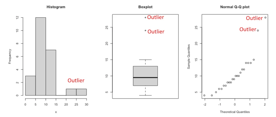
Outlier is an unusual observation that is not consistent with the remaining observations in a sample dataset.
The outliers in a dataset can come from the following possible sources: - contaminated data samples, - data points from different population, - incorrect sampling methods, - underlying significant treatment response, - error in data collection or analysis.
Outliers can largely influence the results of the statistical tests and hence it is necessary to find the outliers in the dataset.
There are several ways how to find outliers!
8.1.2 Using statistics
The first step to detect outliers in R is to start with some descriptive statistics, and in particular with the minimum and maximum.
In R, this can easily be done with the summary() function:
The Standard deviation (SD) and mean of the data can be used for finding the outliers in the dataset. The minimum (Tmin) and maximum (Tmax) threshold based on mean and SD for identifying outliers is given as,
Mean and Standard deviation (SD) outlier formula:
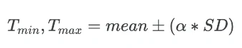
Where α is the threshold factor for defining the number of SD. Generally, the data point which is 3 (α = 3) SD away from the mean is considered as an outlier.
This method works well if the data is normally distributed and when there are very less percentages of outliers in the dataset. It is also sensitive to outliers as mean and SD will change if the outlier is present.
The other variant of the SD method is to use the Clever Standard deviation (Clever SD) method, which is an iterative process to remove outliers. In each iteration, the outlier is removed, and recalculate the mean and SD until no outlier is found. This method uses the threshold factor of 2.5
8.1.3 Using MAD
The median of the dataset can be used in finding the outlier. Median is more robust to outliers as compared to mean.
As opposed to mean, where the standard deviation is used for outlier detection, the median is used in Median Absolute Deviation (MAD) method for outlier detection.
MAD is calculated as:
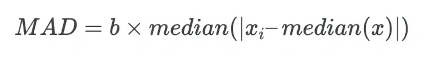
Where b is the scale factor and its value set as 1.4826 when data is normally distributed.
Now, MAD value is used for calculating the threshold values for outlier detection:
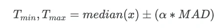
Where, Tmin and Tmax are the minimum and maximum threshold for finding the outlier, and α is a factor for defining the number of MAD. Generally, the data point which is 3 (α = 3) MAD away from the median is considered as an outlier.
This method is more effective than the SD method for outlier detection, but this method is also sensitive, if the dataset contains more than 50% of outliers or 50% of the data contains the same values.
8.1.4 Interquartile Range (IQR)
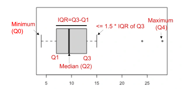
The interquartile range (IQR) is a difference between the data points which ranks at 25th percentile (first quartile or Q1) and 75th percentile (third quartile or Q3) in the dataset (IQR = Q3 - Q1).
The IQR value is used for calculating the threshold values for outlier detection:
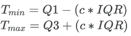
Where, Tmin and Tmax are the thresholds for finding the outlier and c is constant which is generally 1.5 (mild outlier) or 3 (extreme outlier).
The data points which are 1.5 IQR away from Q1 and Q3 are considered as outliers. IQR method is useful when the data does not follow a normal distribution.
Create horizontal boxplot to understand IQR:
8.1.5 Grubb’s Test
Grubb’s test is used for identifying a single outlier (minimum or maximum value in a dataset) in a univariate dataset.
Before performing the test, the set of experimental results (statistical sample) is ranked according to increasing values. A fatal error may be burdened with the highest or lowest value of the result in the sample. For these results, parameters are calculated accordingly Tmax i Tmin.
The parameter with a larger value is then compared with the critical parameter of the Grubbs test, corresponding to the size of the statistical sample and the selected level of confidence. The critical value of the statistics of this test is calculated on the basis of paramter t of the Student distribution for the given confidence level and the number of degrees of freedom (n - 2, n - number of measurements in the series). If the experimental value is greater than the critical value, then the suspected result is burdened with a gross error and can be rejected with a given confidence level.
Null hypothesis (H0): The maximum or minimum value is not an outlier (there is no outlier)
Alternate hypothesis (Ha): The maximum or minimum value is an outlier (there is an outlier)
The null hypothesis is rejected when the G statistics is greater than the critical G value (theoretical G which is expected to occur at a 5% significance level and given sample size).
Test statistic:
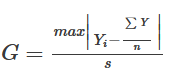
where s - standard deviation.
It is a two-sided test, but it can also be used as a one-sided test then we check: - whether the minimum value is not an outlier - whether the maximum value is an outlier
If you have more than one outlier in the dataset, then you can perform multiple tests to remove outliers. You need to remove the outlier identified in each step and repeat the process.
8.1.6 Tools in R
You will find many other methods to detect outliers:
- in the
outlierspackages, - via the
lofactor()function from theDMwRpackage: Local Outlier Factor (LOF) is an algorithm used to identify outliers by comparing the local density of a point with that of its neighbors, - the
outlierTest()from thecarpackage gives the most extreme observation based on the given model and allows to test whether it is an outlier, - in the
OutlierDetectionpackage, and with theaq.plot()function from themvoutlier.
8.2 Leverage
A data point has high leverage if it has “extreme” predictor x values. With a single predictor, an extreme x value is simply one that is particularly high or low.
With multiple predictors, extreme x values may be particularly high or low for one or more predictors, or may be “unusual” combinations of predictor values (e.g., with two predictors that are positively correlated, an unusual combination of predictor values might be a high value of one predictor paired with a low value of the other predictor).
A data point has high leverage, if it has extreme predictor x values. This can be detected by examining the leverage statistic or the hat-value.
A value of this statistic above 2(p + 1)/n indicates an observation with high leverage (P. Bruce and Bruce 2017); where, p is the number of predictors and n is the number of observations.
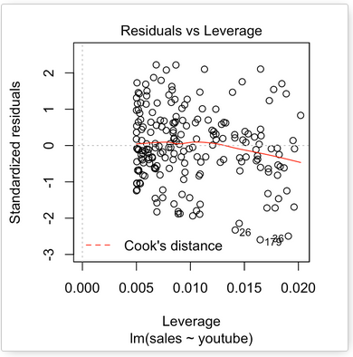
The plot above highlights the top 3 most extreme points (#26, #36 and #179), with a standardized residuals below -2. However, there is no outliers that exceed 3 standard deviations, what is good.
Additionally, there is no high leverage point in the data. That is, all data points, have a leverage statistic below 2(p + 1)/n = 4/200 = 0.02.
8.3 Influential
An influential value is a value, which inclusion or exclusion can alter the results of the regression analysis. Such a value is associated with a large residual.
Not all outliers (or extreme data points) are influential in linear regression analysis.
Statisticians have developed a metric called Cook’s distance to determine the influence of a value. This metric defines influence as a combination of leverage and residual size.
A rule of thumb is that an observation has high influence if Cook’s distance exceeds 4/(n - p - 1)(P. Bruce and Bruce 2017), where n is the number of observations and p the number of predictor variables.
The Residuals vs Leverage plot can help us to find influential observations if any. On this plot, outlying values are generally located at the upper right corner or at the lower right corner. Those spots are the places where data points can be influential against a regression line.
The following plots illustrate the Cook’s distance and the leverage of our model:
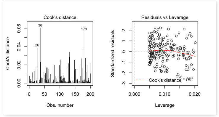
When data points have high Cook’s distance scores and are to the upper or lower right of the leverage plot, they have leverage meaning they are influential to the regression results. The regression results will be altered if we exclude those cases.
On the plots above, the data don’t present any influential points. Cook’s distance lines (a red dashed line) are not shown on the Residuals vs Leverage plot because all points are well inside of the Cook’s distance lines.
Let’s take a look at another example:
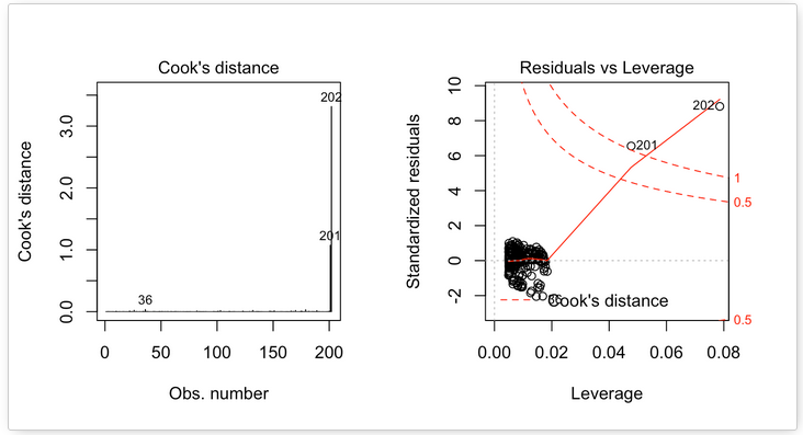
On the Residuals vs Leverage plot, look for a data point outside of a dashed line, Cook’s distance. When the points are outside of the Cook’s distance, this means that they have high Cook’s distance scores. In this case, the values are influential to the regression results. The regression results will be altered if we exclude those cases.
In the above example, two data points are far beyond the Cook’s distance lines. The other residuals appear clustered on the left. The plot identified the influential observation as #201 and #202. If you exclude these points from the analysis, the slope of the regression model coefficient will change! Pretty big impact!
Please take a look also at the tutorial of Unusual Observations Detection here.