Chapter 7 Caring for your document

Once you have your published doc in place, it’s likely that you will want to change it sooner or later. The key to updating is that you must 🧶 Knit each time before you push to GitHub–otherwise your changes won’t be published. This sounds easy enough, but trust us, it is also easy enough to forget!

Here’s what the change-my-doc workflow looks like for me:

1. Open the existing RStudio project
2. 🧶 Knit right away to see where things left off, or turn on xaringan::inf_mr() to see a live preview of your changes.
3. Make edits, preview changes, rinse and repeat…
4. Commit and push all changes to GitHub.

7.1 Live editing

Whenever you are editing a single R Markdown file, and outputting to HTML format, you can turn on “live reload” while you work. This means that, after turning it on, every time you Save your updated output re-renders in your RStudio viewer pane, and also in a browser window if you open it up.

Figure 7.1: Demo of R Markdown live reload from Yihui Xie

To turn on “live reload”, you’ll first need to install the xaringan package²:

install.packages("xaringan")

Then close RStudio.

When you reopen RStudio, in your “Addins” dropdown, scroll down to the bottom where the xaringan addins are. You should see “Infinite Moon Reader”.

The same thing can be accomplished from your R console by running this code:

xaringan::inf_mr()

Now, make a small change to your document, save, and watch the preview reload!

You’ll need to save this file first, before using the “Infinite Moon Reader”.

7.2 Care for your code

7.2.1 Use keyboard shortcuts

To insert R code chunks, you can use the button, or you could use keyboard shortcuts

the keyboard shortcut Ctrl + Alt + I (OS X: Cmd + Option + I)

7.2.2 Add a setup code chunk

Get into the habit of always having your first knitr code chunk be a setup chunk using knitr::opts_chunk$set(). A good one looks like this:

```{r setup, include = FALSE}
knitr::opts_chunk$set(
  comment = "#>",
  fig.path = "figs" # use only for single Rmd files
  collapse = TRUE,
)
```

Inside the parentheses, list the chunk option on the left = a new default value on the right. Each chunk option is separated by a comma. The chunk option for the setup chunk itself is typically include=FALSE so that no one sees it but you.

A few notes on what the above chunk options do:

• comment = "#>" sets the character on the far left of all printed output such that a reader could copy/paste a block of code into their console and run it (they won’t be bombarded by errors produced if they accidentally include your printed output in their code)

• fig.path = "something-here-in-quotes" ensures that all figures that you create with R code all get stored in the folder you name here; this helps if you need to pull up a figure file quickly without needing to explicitly export each individual figure. Read more here.

• collapse = TRUE fuses your code and output together for all code chunks throughout your document.

  Below is a side-by-side changing this chunk option for an individual chunk.

Default chunk style

library(tidyverse)
starwars %>% 
  count(homeworld, sort = TRUE)

## # A tibble: 49 × 2
##    homeworld     n
##    <chr>     <int>
##  1 Naboo        11
##  2 Tatooine     10
##  3 <NA>         10
##  4 Alderaan      3
##  5 Coruscant     3
##  6 Kamino        3
##  7 Corellia      2
##  8 Kashyyyk      2
##  9 Mirial        2
## 10 Ryloth        2
## # … with 39 more rows

Custom chunk style

library(tidyverse)
starwars %>% 
  count(homeworld, sort = TRUE)
#> # A tibble: 49 × 2
#>    homeworld     n
#>    <chr>     <int>
#>  1 Naboo        11
#>  2 Tatooine     10
#>  3 <NA>         10
#>  4 Alderaan      3
#>  5 Coruscant     3
#>  6 Kamino        3
#>  7 Corellia      2
#>  8 Kashyyyk      2
#>  9 Mirial        2
#> 10 Ryloth        2
#> # … with 39 more rows

Our setup code chunk above affects all code chunks. It is called a global chunk option for that reason. You can (and should) use individual chunk options too, but setting up some nice ones that apply to all code chunks can save you time and can lessen your cognitive load as you create your content.

7.2.3 Name your code chunks

Remember how we advised you set your fig.path? One of the best things you can do for yourself is to name your code chunks.

h/t to Maëlle Salmon

Maëlle wrote a fun blog post that (hopefully) will convince you that your chunks are pets rather than livestock (so they deserve a name!).

In short, here are a few very good reasons to name your pets:

1. Easier to find them (use the chunk outline thingie in IDE)
2. Easier to debug when you 🧶 Knit
3. your figures get named!!

We recommend using dashes (-) in chunk labels instead of spaces or underscores (or really, any punctuation)…

✔️ Good

```{r my-dog-skip}

```

❌ Bad

```{r my_dog_skip}

```

7.2.4 Print pretty packages

If you load packages, we recommend setting that code chunk to be message = FALSE, warning = FALSE

```{r, message = FALSE, warning = FALSE}
library(tidyverse)
library(janitor)
```

7.3 Care for your self

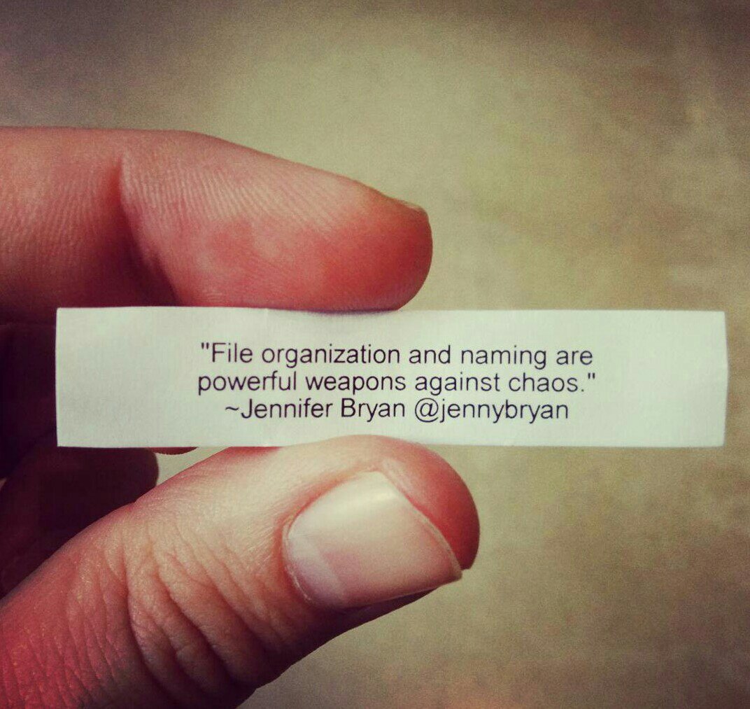
7.3.1 Use portable file paths

When you are in an .Rproj, you’ll probably want to create some directories like data/, images/, figures/, etc. We strongly encourage you to use the here package to build up safe file paths. Read more from Jenny Bryan’s What They Forgot to Teach You About R workshop.

If you are still skeptical, read Malcolm Barret’s blog post Why should I use the here package when I’m already using projects?

Figure 7.2: Artwork by Allison Horst

“The chance of the setwd() command having the desired effect – making the file paths work – for anyone besides its author is 0%.”

— Jenny Bryan

7.3.2 Name your files nicely

https://twitter.com/DGuarch/status/663049353007931392?s=20

7.3.3 Add notes to self

also include how to leave invisible notes to yourself <!--- your comment --->

---

2. xaringan is an R package for making presentation slides with R Markdown↩︎

---

All illustrations CC-BY-NC : You can download them by clicking here
All other materials CC-BY unless noted otherwise.