Chapter 21 Time Series Models
21.1 Univariate Time Series Modeling
Any metric that is measured over regular time intervals forms a time series.
Analysis of time series is commercially importance because of industrial need and relevance especially w.r.t forecasting (demand,sales, supply etc).
In this chapter we will consider fundamental issues related to time series models like:
- Naive models
- Linear models
- ETS models
- Seasonal and non-seasonal ARIMA models
21.2 Time series CHEAT-SHEET
Just to sum up, before we will continue, please take a look at the most popular functions that can help you handle time series :-)
21.2.3 Seasonality
ggseasonplot(myts)# Create a seasonal plot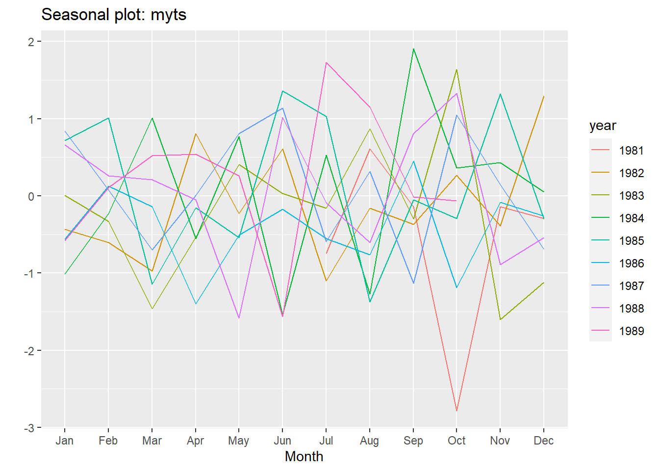
ggsubseriesplot(myts)# Create mini plots for each season and show seasonal means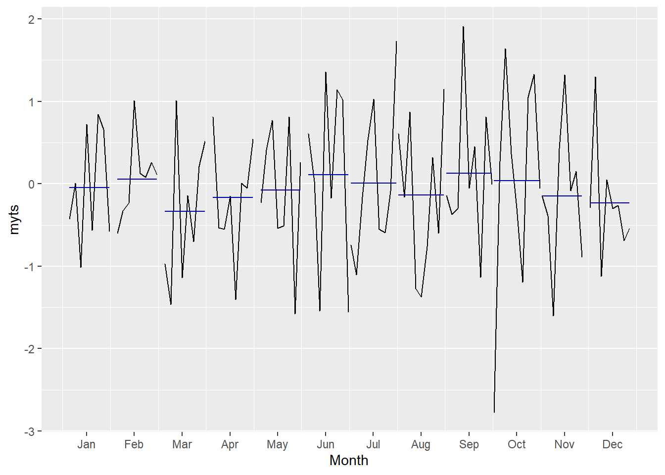
21.2.4 Lags and ACF, PACF
gglagplot(myts)# Plot the time series against lags of itself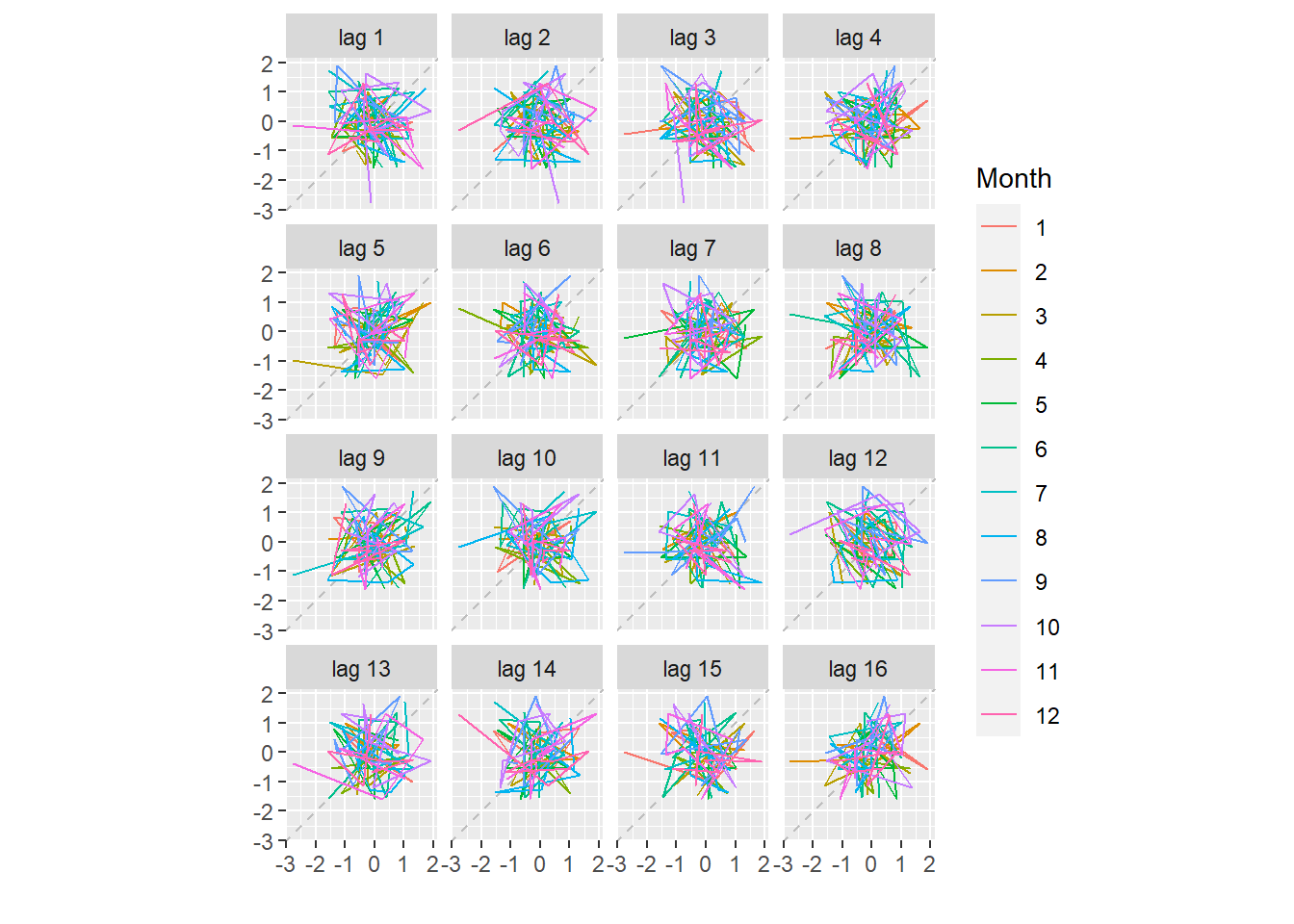
ggAcf(myts)# Plot the autocorrelation function (ACF)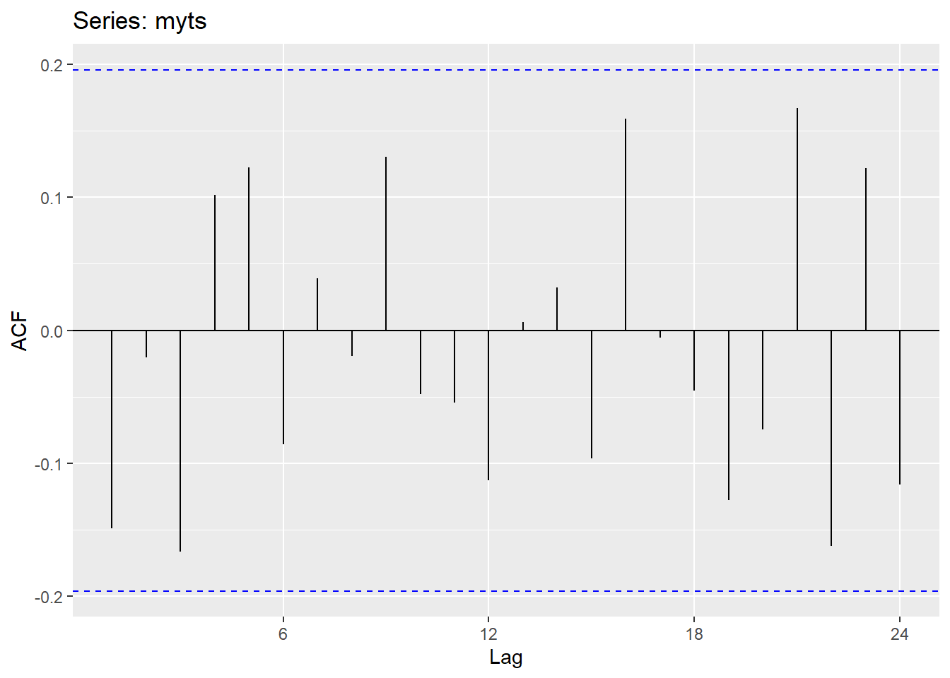
ggPacf(myts)# Plot the partial autocorrelation function (PACF)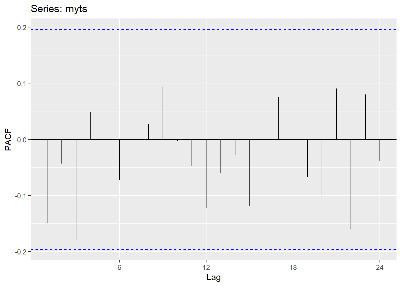
21.2.5 White Noise and the Ljung-Box Test
White Noise is another name for a time series of iid data. Purely random. Ideally your model residuals should look like white noise.
You can use the Ljung-Box test to check if a time series is white noise, here is an example with 24 lags:
Box.test(myts, lag = 24, type="Lj")##
## Box-Ljung test
##
## data: myts
## X-squared = 31, df = 24, p-value = 0.2p-value > 0.05 suggests data are not significantly different than white noise
21.2.6 Model Selection
The forecast package includes a few common models out of the box. Fit the model and create a forecast object, and then use the forecast() function on the object and a number of h periods to predict.
Example of the workflow:
train <- window(data, start = 1980)
fit <- naive(train)
checkresiduals(fit)
pred <- forecast(fit, h=4)
accuracy(pred, data)21.2.8 Residuals
Residuals are the difference between the model`s fitted values and the actual data. Residuals should look like white noise and be:
- Uncorrelated
- Have mean zero
And ideally have:
- Constant variance
- A normal distribution
checkresiduals(): helper function to plot the residuals, plot the ACF and histogram, and do a Ljung-Box test on the residuals.21.2.9 Evaluating Model Accuracy
Train/Test split with window function:
window(data, start, end): to slice the ts dataUse accuracy() on the model and test set:
accuracy(model, testset): Provides accuracy measures like MAE, MSE, MAPE, RMSE etcBacktesting with one step ahead forecasts, aka Time series cross validation can be done with a helper function tsCV().
tsCV(): returns forecast errors given a forecastfunction that returns a forecast object and number of steps ahead h. At h = 1 the forecast errors will just be the model residuals.Here`s an example using the naive() model, forecasting one period ahead:
tsCV(data, forecastfunction = naive, h = 1)21.2.10 Many Models
Exponential Models
- ses(): Simple Exponential Smoothing, implement a smoothing parameter alpha on previous data
- holt(): Holt`s linear trend, SES + trend parameter. Use damped=TRUE for damped trending
- hw(): Holt-Winters method, incorporates linear trend and seasonality. Set seasonal=
additivefor additive version ormultiplicativefor multiplicative version
ETS Models
The forecast package includes a function ets() for your exponential smoothing models. ets() estimates parameters using the likelihood of the data arising from the model, and selects the best model using corrected AIC (AICc) * Error = {A, M} * Trend = {N, A, Ad} * Seasonal = {N, A, M}
ARIMA
Arima(): Implementation of the ARIMA function, set include.constant = TRUE to include drift aka the constant
auto.arima(): Automatic implentation of the ARIMA function in forecast. Estimates parameters using maximum likelihood and does a stepwise search between a subset of all possible models. Can take a lambda argument to fit the model to transformed data and the forecasts will be back-transformed onto the original scale. Turn stepwise = FALSE to consider more models at the expense of more time.
TBATS
Automated model that combines exponential smoothing, Box-Cox transformations, and Fourier terms. Pro: Automated, allows for complex seasonality that changes over time. Cons: Slow.
- T: Trigonometric terms for seasonality
- B: Box-Cox transformations for heterogeneity
- A: ARMA errors for short term dynamics
- T: Trend (possibly damped)
- S: Seasonal (including multiple and non-integer periods)
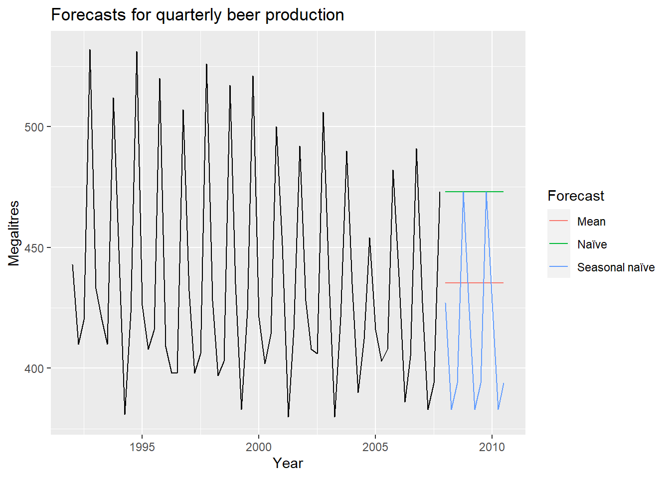
21.3 Naive approach
Using the naive method, all forecasts for the future are equal to the last observed value of the series. Naive forecasts are where all forecasts are simply set to be the value of the last observation. That is, \[ \hat{y}_{T+h|T} = y_{T}. \] This method works remarkably well for many economic and financial time series.
Using the average method, all future forecasts are equal to a simple average of the observed data. Here, the forecasts of all future values are equal to the mean of the historical data. If we let the historical data be denoted by \(y_{1},\dots,y_{T}\), then we can write the forecasts as \[ \hat{y}_{T+h|T} = \bar{y} = (y_{1}+\dots+y_{T})/T. \] The notation \(\hat{y}_{T+h|T}\) is a short-hand for the estimate of \(y_{T+h}\) based on the data \(y_1,\dots,y_T\).
21.3.1 Seasonal naive method
A similar method is useful for highly seasonal data. In this case, we set each forecast to be equal to the last observed value from the same season of the year (e.g., the same month of the previous year). Formally, the forecast for time \(T+h\) is written as \[ \hat{y}_{T+h|T} = y_{T+h-km}, \] where \(m=\) the seasonal period, \(k=\lfloor (h-1)/m\rfloor+1\), and \(\lfloor u \rfloor\) denotes the integer part of \(u\). That looks more complicated than it really is.
For example, with monthly data, the forecast for all future February values is equal to the last observed February value. With quarterly data, the forecast of all future Q2 values is equal to the last observed Q2 value (where Q2 means the second quarter). Similar rules apply for other months and quarters, and for other seasonal periods.
21.3.2 Drift method
A variation on the naive method is to allow the forecasts to increase or decrease over time, where the amount of change over time (called the “drift”) is set to be the average change seen in the historical data. Thus the forecast for time \(T+h\) is given by \[ \hat{y}_{T+h|T} = y_{T} + \frac{h}{T-1}\sum_{t=2}^T (y_{t}-y_{t-1}) = y_{T} + h \left( \frac{y_{T} -y_{1}}{T-1}\right). \] This is equivalent to drawing a line between the first and last observations, and extrapolating it into the future.
21.4 Linear models
21.4.1 Multiple regression
\[ y_t = \beta_0 + \beta_1 x_{1,t} + \beta_2 x_{2,t} + \cdots + \beta_kx_{k,t} + \varepsilon_t. \]
- \(y_t\) is the variable we want to predict: the response variable
- Each \(x_{j,t}\) is numerical and is called a predictor. They are usually assumed to be known for all past and future times.
- The coefficients \(\beta_1,\dots,\beta_k\) measure the effect of each predictor after taking account of the effect of all other predictors in the model. That is, the coefficients measure the marginal effects.
- \(\varepsilon_t\) is a white noise error term
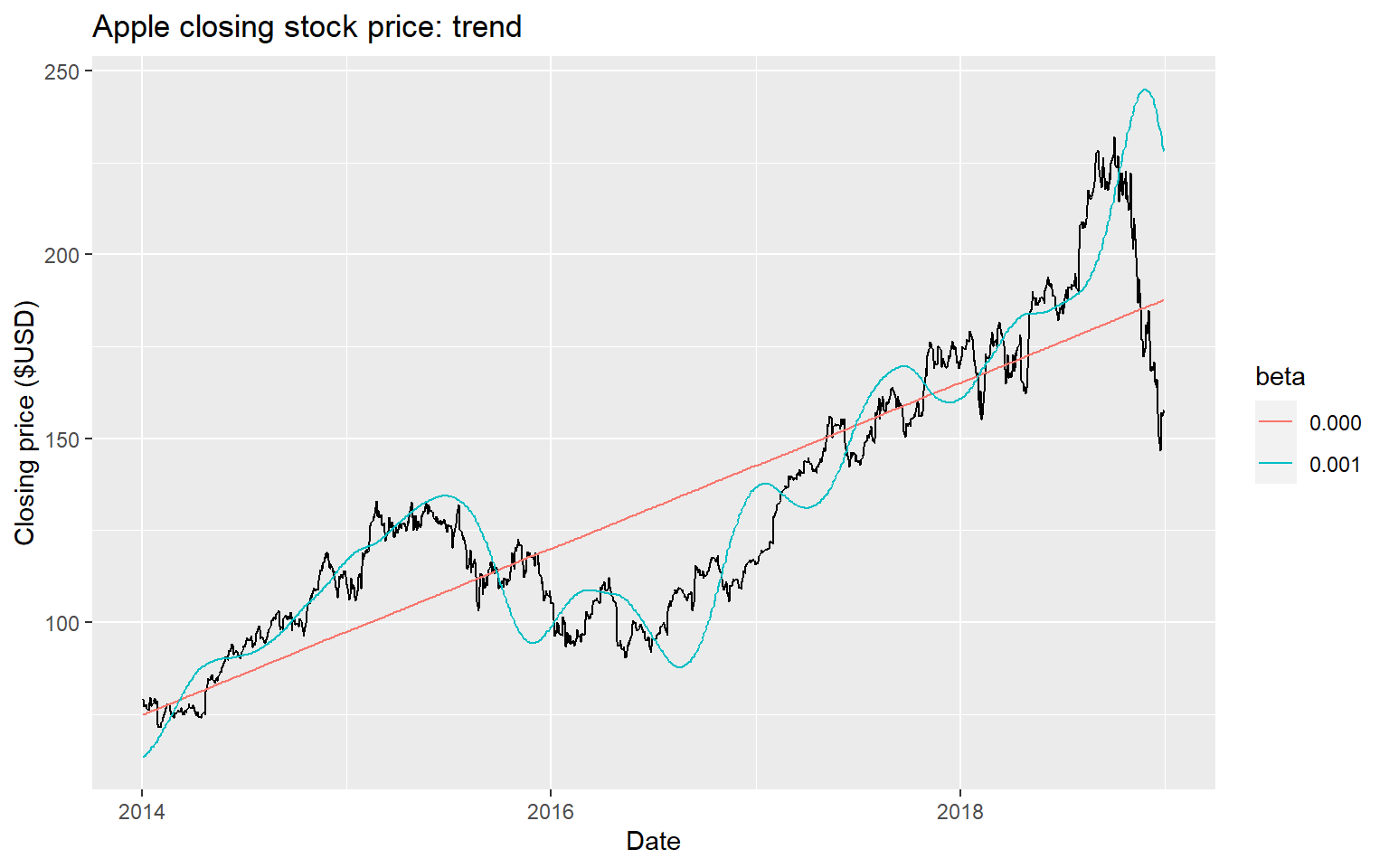
21.4.3 Trend
Linear trend \[ x_t = t \]
- \(t=1,2,\dots,T\)
- Strong assumption that trend will continue.
Seasonal dummies
- For quarterly data: use 3 dummies
- For monthly data: use 11 dummies
- For daily data: use 6 dummies
- What to do with weekly data?
Outliers
- If there is an outlier, you can use a dummy variable (taking value 1 for that observation and 0 elsewhere) to remove its effect.
Public holidays
- For daily data: if it is a public holiday, dummy=1, otherwise dummy=0.
21.4.4 Beer production - example
Regression model: \[ y_t = \beta_0 + \beta_1 t + \beta_2d_{2,t} + \beta_3 d_{3,t} + \beta_4 d_{4,t} + \varepsilon_t \]
- \(d_{i,t} = 1\) if \(t\) is quarter \(i\) and 0 otherwise.
- The first quarter variable has been omitted, so the coefficients associated with the other quarters are measures of the difference between those quarters and the first quarter.
fit.beer <- tslm(fpp::ausbeer ~ trend + season)
summary(fit.beer)
##
## Call:
## tslm(formula = fpp::ausbeer ~ trend + season)
##
## Residuals:
## Min 1Q Median 3Q Max
## -107.66 -50.64 -9.02 44.54 134.20
##
## Coefficients:
## Estimate Std. Error t value Pr(>|t|)
## (Intercept) 335.4871 10.7323 31.26 < 2e-16 ***
## trend 0.7754 0.0668 11.60 < 2e-16 ***
## season2 -45.5679 11.4848 -3.97 0.0001 ***
## season3 -31.6829 11.4854 -2.76 0.0063 **
## season4 67.6651 11.5399 5.86 1.8e-08 ***
## ---
## Signif. codes: 0 '***' 0.001 '**' 0.01 '*' 0.05 '.' 0.1 ' ' 1
##
## Residual standard error: 59.1 on 206 degrees of freedom
## Multiple R-squared: 0.547, Adjusted R-squared: 0.538
## F-statistic: 62.1 on 4 and 206 DF, p-value: <2e-16There is an average downward trend of -0.34 megalitres per quarter. On average, the second quarter has production of 34.7 megalitres lower than the first quarter, the third quarter has production of 17.8 megalitres lower than the first quarter, and the fourth quarter has production of 72.8 megalitres higher than the first quarter.
autoplot(fpp::ausbeer, series="Data") +
  autolayer(fitted(fit.beer), series="Fitted") +
  xlab("Year") + ylab("Megalitres") +
  ggtitle("Quarterly Beer Production")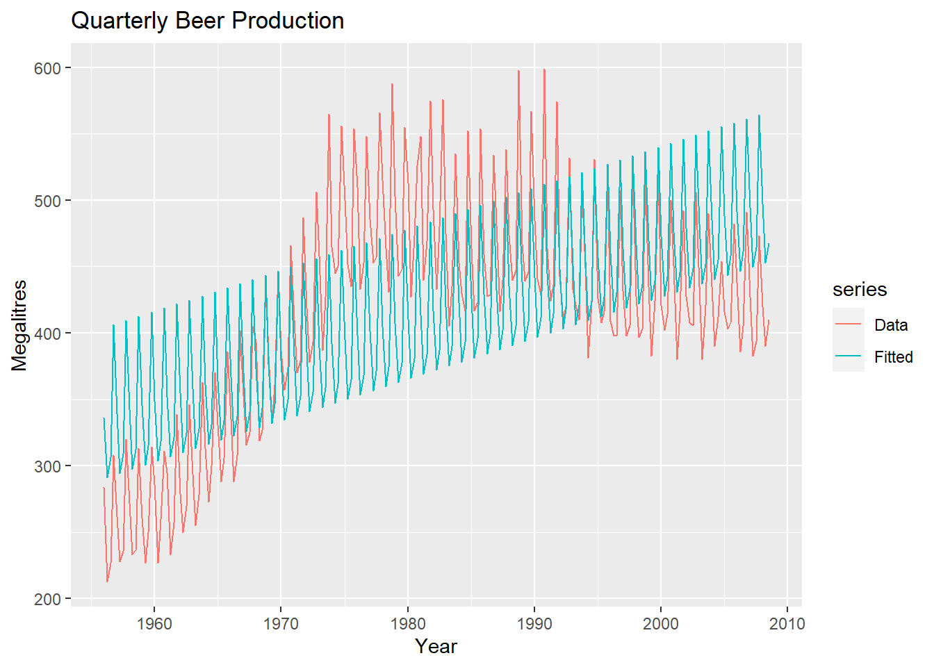
Now we can run the diagnostics (OLS!):
checkresiduals(fit.beer, test=FALSE)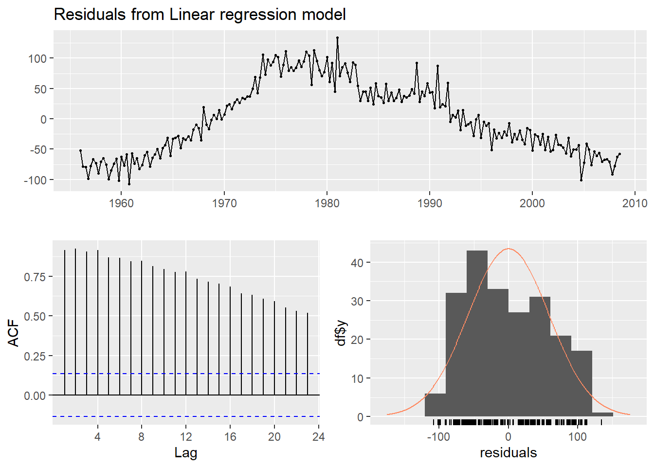
21.5 ETS models
21.5.1 Historical perspective
- Developed in the 1950s and 1960s as methods (algorithms) to produce point forecasts.
- Combine a level, trend (slope) and seasonal component to describe a time series.
- The rate of change of the components are controlled by smoothing parameters: \(\alpha\), \(\beta\) and \(\gamma\) respectively.
- Need to choose best values for the smoothing parameters (and initial states).
- Equivalent ETS state space models developed in the 1990s and 2000s.
21.5.2 Simple method
- Simple exponential smoothing is suitable for forecasting data with no clear trend or seasonal pattern.
- Exponential smoothing was proposed in the late 1950s(Brown, 1959; Holt, 1957; Winters, 1960), and has motivated some of the most successful forecasting methods.
- Forecasts produced using exponential smoothing methods are weighted averages of past observations, with the weights decaying exponentially as the observations get older.
- In other words, the more recent the observation the higher the associated weight:
\[ \begin{aligned} \hat{y}_{y}^{*}={\alpha}{y_{t-1}}+(1-\alpha)\hat{y}_{t1} \end{aligned} \]
- Want something in between that weights most recent data more highly.
- Simple exponential smoothing uses a weighted moving average with weights that decrease exponentially!
21.5.3 Optimisation
- The application of every exponential smoothing method requires the smoothing parameters and the initial values to be chosen.
- A more reliable and objective way to obtain values for the unknown parameters is to estimate them from the observed data.
- The unknown parameters and the initial values for any exponential smoothing method can be estimated by minimising the SSE.
21.5.4 ETS models with trend
The Holt`s exponential smoothing approach can fit a time series that has an overall level and a trend (slope)
\(b_t\): slope
State space form: \[ \begin{aligned} y_t&=\ell_{t-1}+b_{t-1}+\varepsilon_t\\ \ell_t&=\ell_{t-1}+b_{t-1}+\alpha \varepsilon_t\\ b_t&=b_{t-1}+\alpha\beta^* \varepsilon_t \end{aligned} \]
For simplicity, set \(\beta=\alpha \beta^*\).
An alpha smoothing parameter controls the exponential decay for the level, and a beta smoothing parameter controls the exponential decay for the slope
Each parameter ranges from 0 to 1, with larger values giving more weight to recent observations
\[ \begin{aligned} \text{Forecast }&& {y}_{t+h|t} &= \ell_{t} + hb_{t} \\ \text{Level }&& \ell_{t} &= \alpha y_{t} + (1 - \alpha)(\ell_{t-1} + b_{t-1})\\ \text{Trend }&& b_{t} &= \beta^*(\ell_{t} - \ell_{t-1}) + (1 -\beta^*)b_{t-1}, \end{aligned} \]
- Two smoothing parameters \(\alpha\) and \(\beta^*\) (\(0\le\alpha,\beta^*\le1\)).
- \(\ell_t\) level: weighted average between \(y_t\) and one-step ahead forecast for time \(t\), \((\ell_{t-1} + b_{t-1}={y}_{t|t-1})\).
- \(b_t\) slope: weighted average of \((\ell_{t} - \ell_{t-1})\) and \(b_{t-1}\), current and previous estimate of slope.
- Choose \(\alpha, \beta^*, \ell_0, b_0\) to minimise SSE.
21.5.5 Holt and Winters model
- The Holt-Winters exponential smoothing approach can be used to fit a time series that has an overall level, a trend, and a seasonal component:
\[ \begin{aligned} \text{Observation equation}&& y_t&=\ell_{t-1}+b_{t-1}+s_{t-m} + \varepsilon_t\\ \text{State equations}&& \ell_t&=\ell_{t-1}+b_{t-1}+\alpha \varepsilon_t\\ && b_t&=b_{t-1}+\beta \varepsilon_t \\ && s_t &= s_{t-m} + \gamma\varepsilon_t \end{aligned} \]
- \(s_t\): seasonal state.
21.5.6 Holt-Winters additive model
\[ \begin{aligned} {y}_{t+h|t} &= \ell_{t} + hb _{t} + s_{t+h-m(k+1)} \\ \ell_{t} &= \alpha(y_{t} - s_{t-m}) + (1 - \alpha)(\ell_{t-1} + b_{t-1})\\ b_{t} &= \beta^*(\ell_{t} - \ell_{t-1}) + (1 - \beta^*)b_{t-1}\\ s_{t} &= \gamma (y_{t}-\ell_{t-1}-b_{t-1}) + (1-\gamma)s_{t-m} \end{aligned} \]
- \(k=\) integer part of \((h-1)/m\).
- Parameters: \(0\le \alpha\le 1\), \(0\le \beta^*\le 1\), \(0\le \gamma\le 1-\alpha\) and \(m=\) period of seasonality (e.g.\(m=4\) for quarterly data).
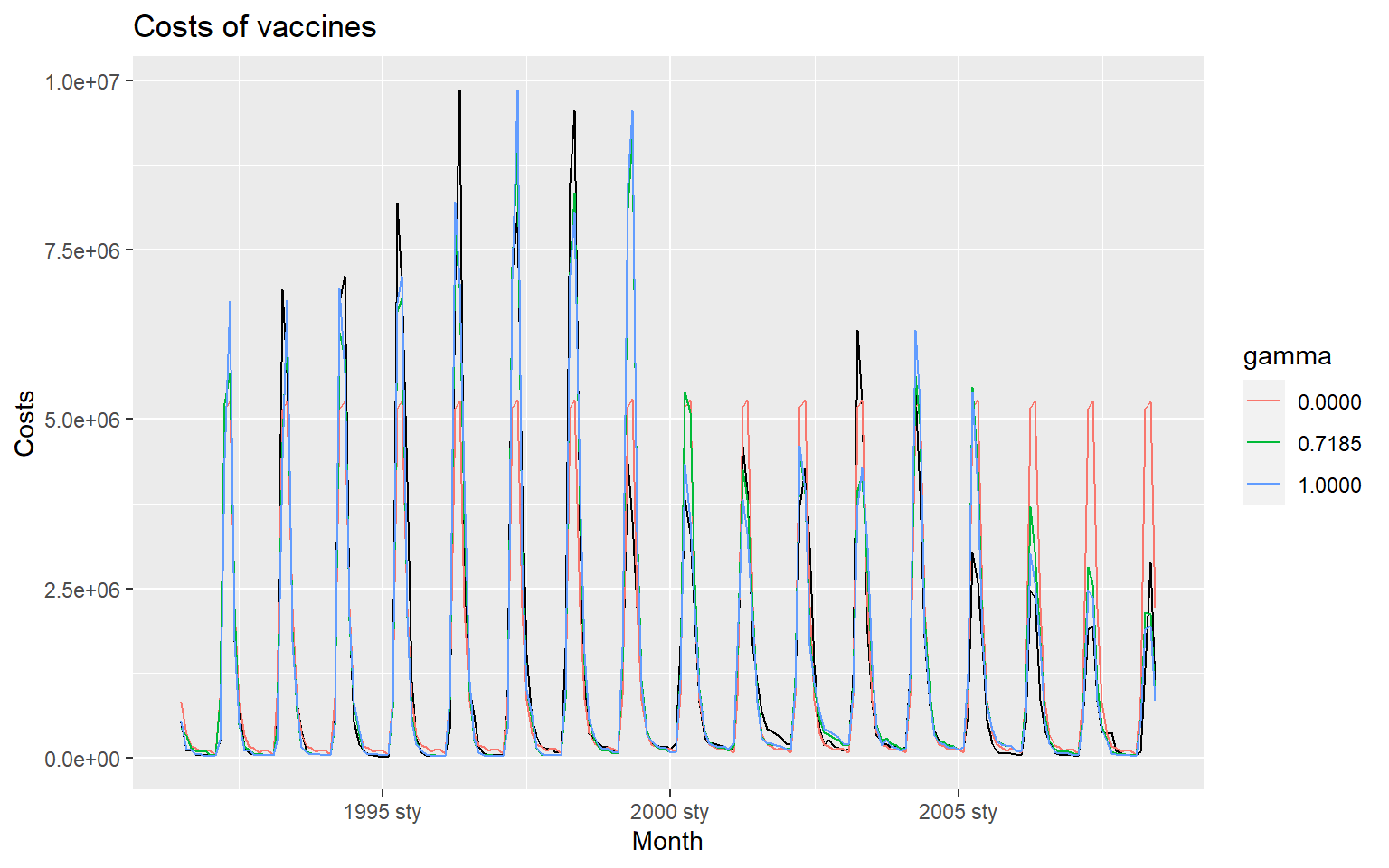
21.5.7 Holt-Winters multiplicative method
- Holt-Winters multiplicative method with multiplicative errors for when seasonal variations are changing proportional to the level of the series.
\[ \begin{aligned} \text{Observation equation}&& y_t&= (\ell_{t-1}+b_{t-1})s_{t-m}(1 + \varepsilon_t)\\ \text{State equations}&& \ell_t&=(\ell_{t-1}+b_{t-1})(1+\alpha \varepsilon_t)\\ && b_t&=b_{t-1}(1+\beta \varepsilon_t) \\ &&s_t &= s_{t-m}(1 + \gamma\varepsilon_t) \end{aligned} \]
- \(k\) is integer part of \((h-1)/m\).
aus_holidays <- tourism %>% filter(Purpose == "Holiday") %>%
  summarise(Trips = sum(Trips))
fit <- aus_holidays %>%
  model(
    additive = ETS(Trips ~ error("A") + trend("A") + season("A")),
    multiplicative = ETS(Trips ~ error("M") + trend("A") + season("M"))
  )
fc <- fit %>% forecast()
fc %>%
autoplot(aus_holidays, level = NULL) + xlab("Year") +
ylab("Variable") +
scale_color_brewer(type = "qual", palette = "Dark2")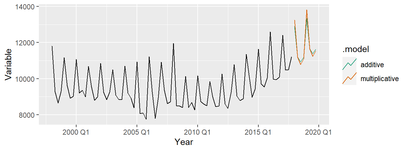
21.6 Autoregressive models
While exponential smoothing models are based on a description of the trend and seasonality in the data, ARIMA models aim to describe the autocorrelations in the data.
Autoregressive (AR) models:
\[ y_{t} = c + \phi_{1}y_{t - 1} + \phi_{2}y_{t - 2} + \cdots + \phi_{p}y_{t - p} + \varepsilon_{t} \] where \(\varepsilon_t\) is white noise. This is a multiple regression with lagged values of \(y_t\) as predictors. Autoregressive models are remarkably flexible at handling a wide range of different time series patterns.
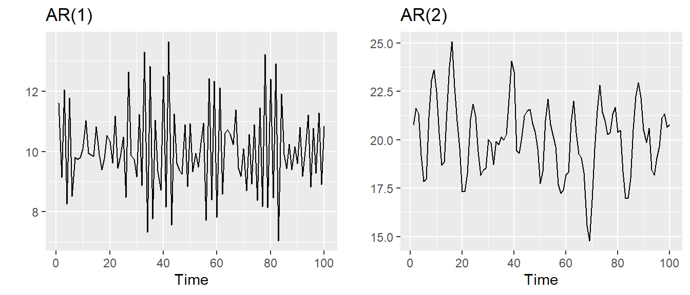
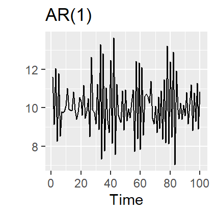
21.6.1 AR(1) model
\(y_{t} = 2 -0.8 y_{t - 1} + \varepsilon_{t}\)
\(\varepsilon_t\sim N(0,1)\),\(T=100\).
\(y_{t} = c + \phi_1 y_{t - 1} + \varepsilon_{t}\)
- When \(\phi_1=0\), \(y_t\) is equivalent to White Noise
- When \(\phi_1=1\) and \(c=0\), \(y_t\) is equivalent to a Random Walk
- When \(\phi_1=1\) and \(c\ne0\), \(y_t\) is equivalent to a Random Walk with drift
- When \(\phi_1<0\), \(y_t\) tends to oscillate between positive and negative values.
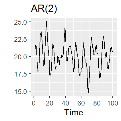
21.6.2 AR(2) model
\(y_t = 8 + 1.3y_{t-1} - 0.7 y_{t-2} + \varepsilon_t\\\)
\(\varepsilon_t\sim N(0,1)\), \(T=100\).
21.6.3 Stationarity conditions
We normally restrict autoregressive models to stationary data, and then some constraints on the values of the parameters are required.
General condition for stationarity: Complex roots of \(1-\phi_1 z - \phi_2 z^2 - \dots - \phi_pz^p\) lie outside the unit circle on the complex plane.
- For \(p=1\): \(-1<\phi_1<1\).
- For \(p=2\): \(-1<\phi_2<1\qquad \phi_2+\phi_1 < 1 \qquad \phi_2 -\phi_1 < 1\).
- More complicated conditions hold for \(p\ge3\).
- Estimation software takes care of this.
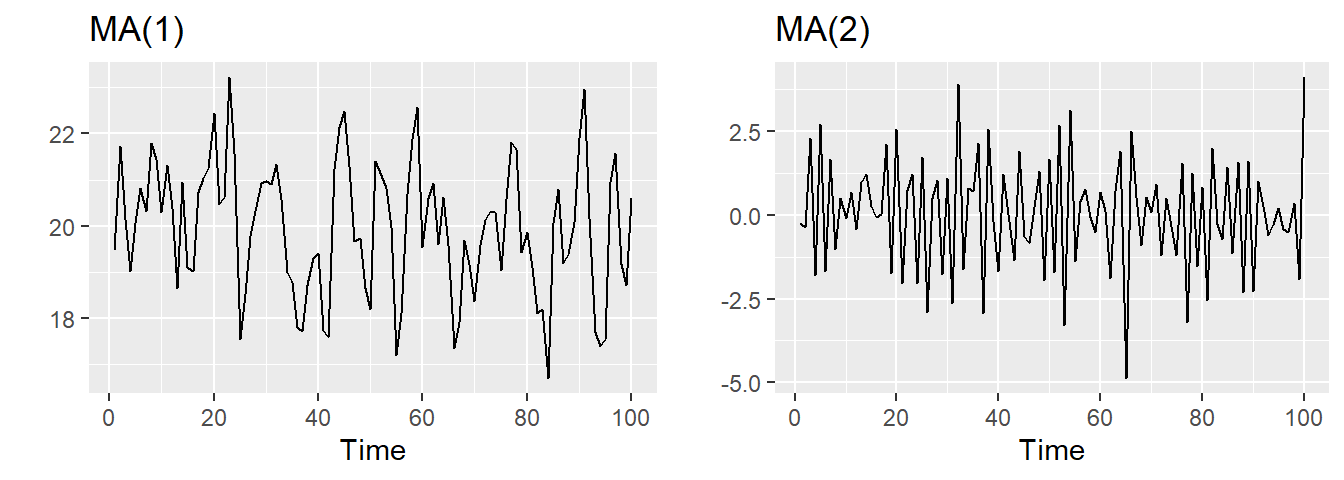
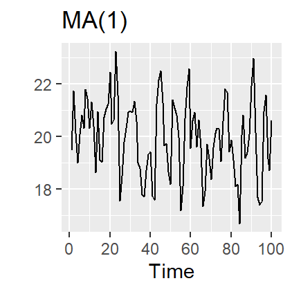
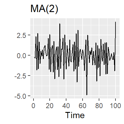
21.7 Moving Average (MA) models
Rather than using past values of the forecast variable in a regression, a moving average model uses past forecast errors in a regression-like model.
Moving Average (MA) models: \[ y_{t} = c + \varepsilon_t + \theta_{1}\varepsilon_{t - 1} + \theta_{2}\varepsilon_{t - 2} + \cdots + \theta_{q}\varepsilon_{t - q}, \]
where \(\varepsilon_t\) is white noise.
This is a multiple regression with past errors as predictors. Don’t confuse this with moving average smoothing!
21.8 ARIMA models
AutoRegressive Moving Average models:
\[ y_{t} = c + \phi_{1}y_{t - 1} + \cdots + \phi_{p}y_{t - p} + \theta_{1}\varepsilon_{t - 1} + \cdots + \theta_{q}\varepsilon_{t - q} + \varepsilon_{t}. \]
- Predictors include both lagged values of \(y_t\) and lagged errors.
- Conditions on coefficients ensure stationarity.
- Conditions on coefficients ensure invertibility.
- Combined ARMA model with differencing.
ARIMA(\(p, d, q\)) model:
AR: \(p =\) order of the autoregressive part
I: \(d =\) degree of first differencing involved
MA: \(q =\) order of the moving average part
White noise model: ARIMA(0,0,0)
Random walk: ARIMA(0,1,0) with no constant
Random walk with drift: ARIMA(0,1,0) with \(\rlap{const.}\)
AR(\(p\)): ARIMA(\(p\),0,0)
MA(\(q\)): ARIMA(0,0,\(q\))
21.8.1 Exercise
Now let`s focus on the retail trade.
autoplot(euretail) +
  xlab("Year") + ylab("Retail index")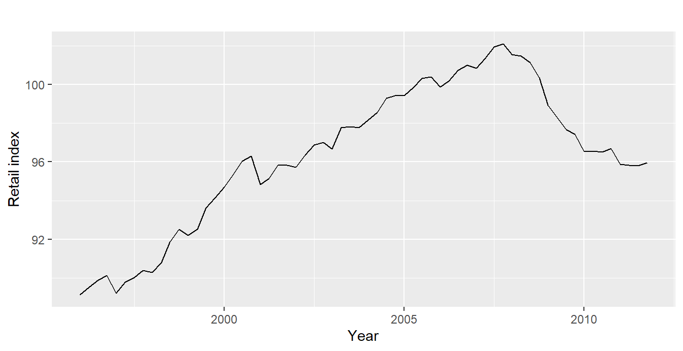
We should probably use some transformations to stabilize the variance.
euretail %>% diff(lag=4) %>% diff() %>%
  ggtsdisplay()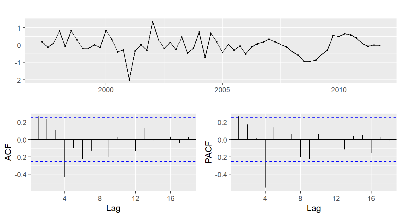
- \(d=1\) and \(D=1\) seems necessary.
- Significant spike at lag 1 in ACF suggests non-seasonal MA(1) component.
- Significant spike at lag 4 in ACF suggests seasonal MA(1) component.
- Initial candidate model: ARIMA(0,1,1)(0,1,1)\(_4\).
- We could also have started with ARIMA(1,1,0)(1,1,0)\(_4\).
fit <- Arima(euretail, order=c(0,1,1),
  seasonal=c(0,1,1))
checkresiduals(fit)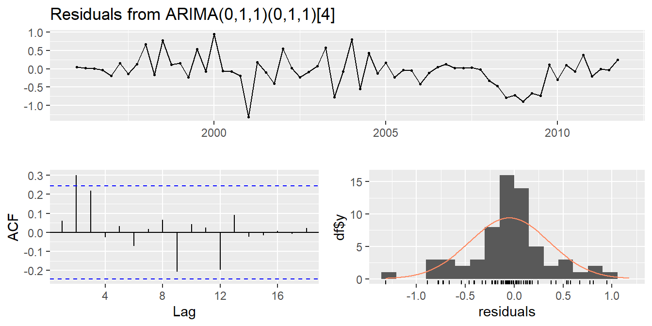
##
##  Ljung-Box test
##
## data:  Residuals from ARIMA(0,1,1)(0,1,1)[4]
## Q* = 11, df = 6, p-value = 0.1
##
## Model df: 2.   Total lags used: 8
##
## Ljung-Box test
##
## data: Residuals from ARIMA(0,1,1)(0,1,1)[4]
## Q* = 11, df = 6, p-value = 0.1
##
## Model df: 2. Total lags used: 8- ACF and PACF of residuals show significant spikes at lag 2, and maybe lag 3.
- AICc of ARIMA(0,1,2)(0,1,1)\(_4\) model is 74.36.
- AICc of ARIMA(0,1,3)(0,1,1)\(_4\) model is 68.53.
fit <- Arima(euretail, order=c(0,1,3),
  seasonal=c(0,1,1))
checkresiduals(fit)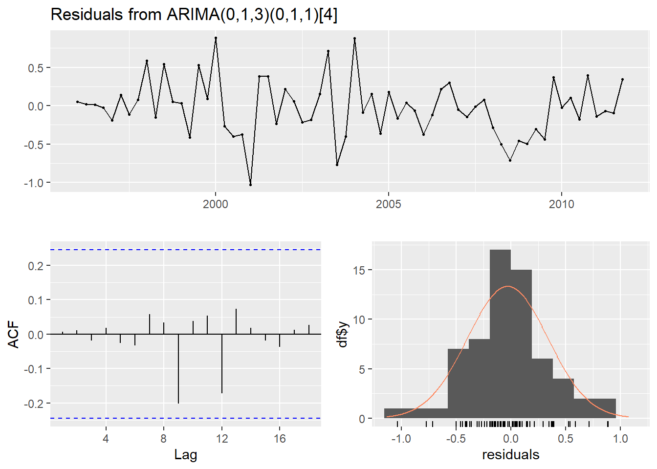
##
##  Ljung-Box test
##
## data:  Residuals from ARIMA(0,1,3)(0,1,1)[4]
## Q* = 0.51, df = 4, p-value = 1
##
## Model df: 4.   Total lags used: 8
(fit <- Arima(euretail, order=c(0,1,3),
seasonal=c(0,1,1)))## Series: euretail
## ARIMA(0,1,3)(0,1,1)[4]
##
## Coefficients:
## ma1 ma2 ma3 sma1
## 0.263 0.370 0.419 -0.661
## s.e. 0.124 0.126 0.130 0.156
##
## sigma^2 = 0.156: log likelihood = -28.7
## AIC=67.4 AICc=68.53 BIC=77.78checkresiduals(fit)
##
##  Ljung-Box test
##
## data:  Residuals from ARIMA(0,1,3)(0,1,1)[4]
## Q* = 0.51, df = 4, p-value = 1
##
## Model df: 4. Total lags used: 8checkresiduals(fit, plot=FALSE)##
## Ljung-Box test
##
## data: Residuals from ARIMA(0,1,3)(0,1,1)[4]
## Q* = 0.51, df = 4, p-value = 1
##
## Model df: 4. Total lags used: 8autoplot(forecast(fit, h=12))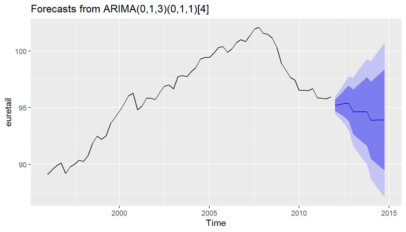
auto.arima(euretail)## Series: euretail
## ARIMA(0,1,3)(0,1,1)[4]
##
## Coefficients:
## ma1 ma2 ma3 sma1
## 0.263 0.370 0.419 -0.661
## s.e. 0.124 0.126 0.130 0.156
##
## sigma^2 = 0.156: log likelihood = -28.7
## AIC=67.4 AICc=68.53 BIC=77.78auto.arima(euretail,
stepwise=FALSE, approximation=FALSE)## Series: euretail
## ARIMA(0,1,3)(0,1,1)[4]
##
## Coefficients:
## ma1 ma2 ma3 sma1
## 0.263 0.370 0.419 -0.661
## s.e. 0.124 0.126 0.130 0.156
##
## sigma^2 = 0.156: log likelihood = -28.7
## AIC=67.4 AICc=68.53 BIC=77.7821.9 Seasonal ARIMA models
A seasonal ARIMA model is formed by including additional seasonal terms in the ARIMA models we have seen so far. The seasonal part of the model consists of terms that are similar to the non-seasonal components of the model, but involve backshifts of the seasonal period.
The modelling procedure is almost the same as for non-seasonal data, except that we need to select seasonal AR and MA terms as well as the non-seasonal components of the model!
| ARIMA | \(~\underbrace{(p, d, q)}\) | \(\underbrace{(P, D, Q)_{m}}\) |
|---|---|---|
| \({\uparrow}\) | \({\uparrow}\) | |
| Non-seasonal part | Seasonal part of | |
| of the model | of the model |
where \(m =\) number of observations per year.
E.g., ARIMA\((1, 1, 1)(1, 1, 1)_{4}\) model (without constant) \[(1 - \phi_{1}B)(1 - \Phi_{1}B^{4}) (1 - B) (1 - B^{4})y_{t} ~= ~ (1 + \theta_{1}B) (1 + \Theta_{1}B^{4})\varepsilon_{t}. \]
All the factors can be multiplied out and the general model written as follows: \begin{align*} y_{t} &= (1 + \phi_{1})y_{t - 1} - \phi_1y_{t-2} + (1 + \Phi_{1})y_{t - 4}\\ &\text{} - (1 + \phi_{1} + \Phi_{1} + \phi_{1}\Phi_{1})y_{t - 5} + (\phi_{1} + \phi_{1} \Phi_{1}) y_{t - 6} \\ & \text{} - \Phi_{1} y_{t - 8} + (\Phi_{1} + \phi_{1} \Phi_{1}) y_{t - 9} - \phi_{1} \Phi_{1} y_{t - 10}\\ &\text{} + \varepsilon_{t} + \theta_{1}\varepsilon_{t - 1} + \Theta_{1}\varepsilon_{t - 4} + \theta_{1}\Theta_{1}\varepsilon_{t - 5}. \end{align*}
21.9.1 Common ARIMA models
The Census Bureaus (in many countries) use the following models most often:
ARIMA(0,1,1)(0,1,1)\(_m\) with log transformation
ARIMA(0,1,2)(0,1,1)\(_m\) with log transformation
ARIMA(2,1,0)(0,1,1)\(_m\) with log transformation
ARIMA(0,2,2)(0,1,1)\(_m\) with log transformation
ARIMA(2,1,2)(0,1,1)\(_m\) with no transformation
The seasonal part of an AR or MA model will be seen in the seasonal lags of the PACF and ACF.
ARIMA(0,0,0)(0,0,1)\(_{12}\) will show:
- a spike at lag 12 in the ACF but no other significant spikes.
- The PACF will show exponential decay in the seasonal lags; that is, at lags 12, 24, 36, etc.
ARIMA(0,0,0)(1,0,0)\(_{12}\) will show:
- exponential decay in the seasonal lags of the ACF
- a single significant spike at lag 12 in the PACF.
21.9.2 Exercise
Lets continue the analysis on the quarterly retail trade:
eu_retail <- as_tsibble(fpp2::euretail)
eu_retail %>% autoplot(value) +
  xlab("Year") + ylab("Retail index")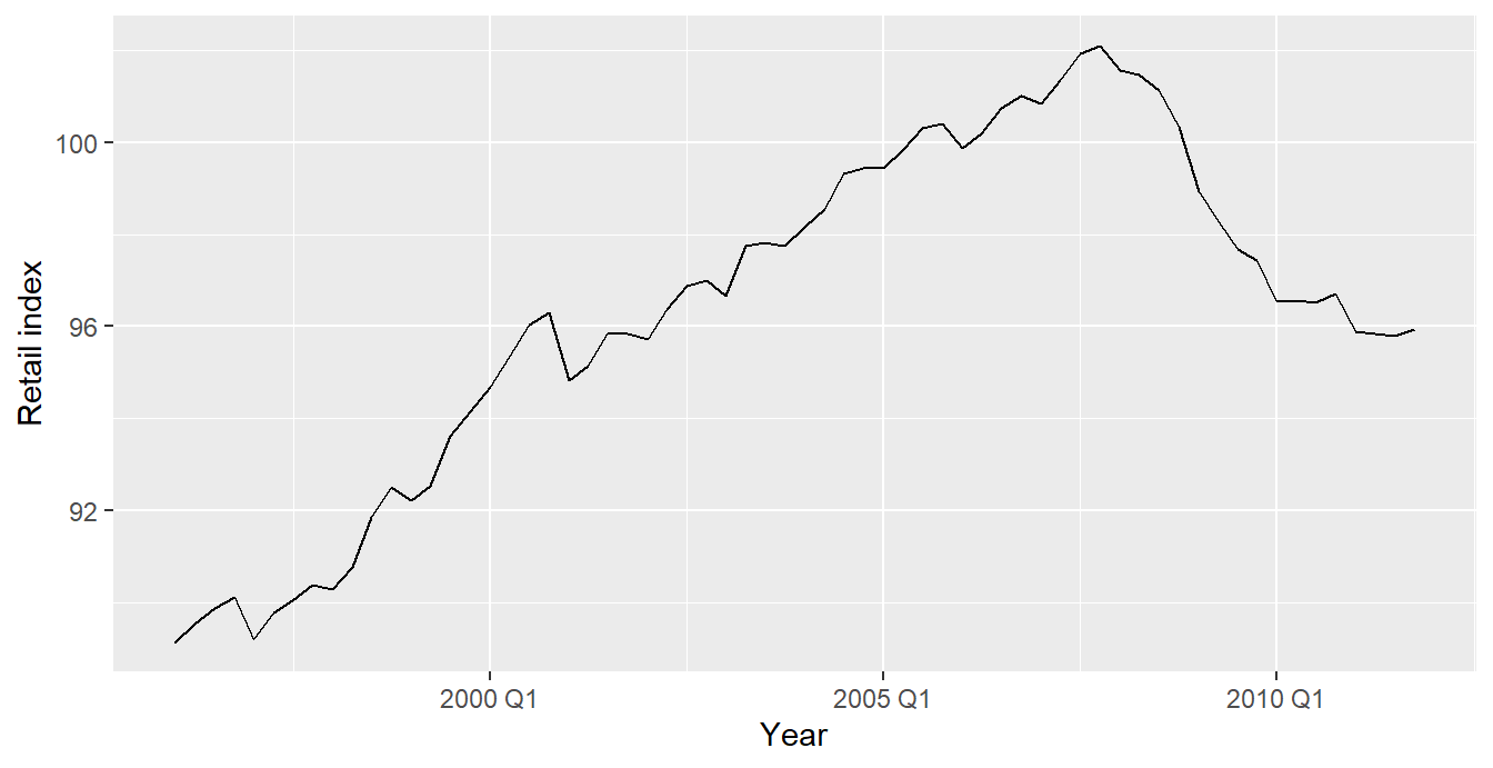
eu_retail %>% gg_tsdisplay(
  value %>% difference(4), plot_type='partial')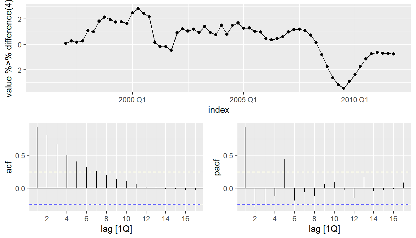
eu_retail %>% gg_tsdisplay(
  value %>% difference(4) %>% difference(1),plot_type='partial')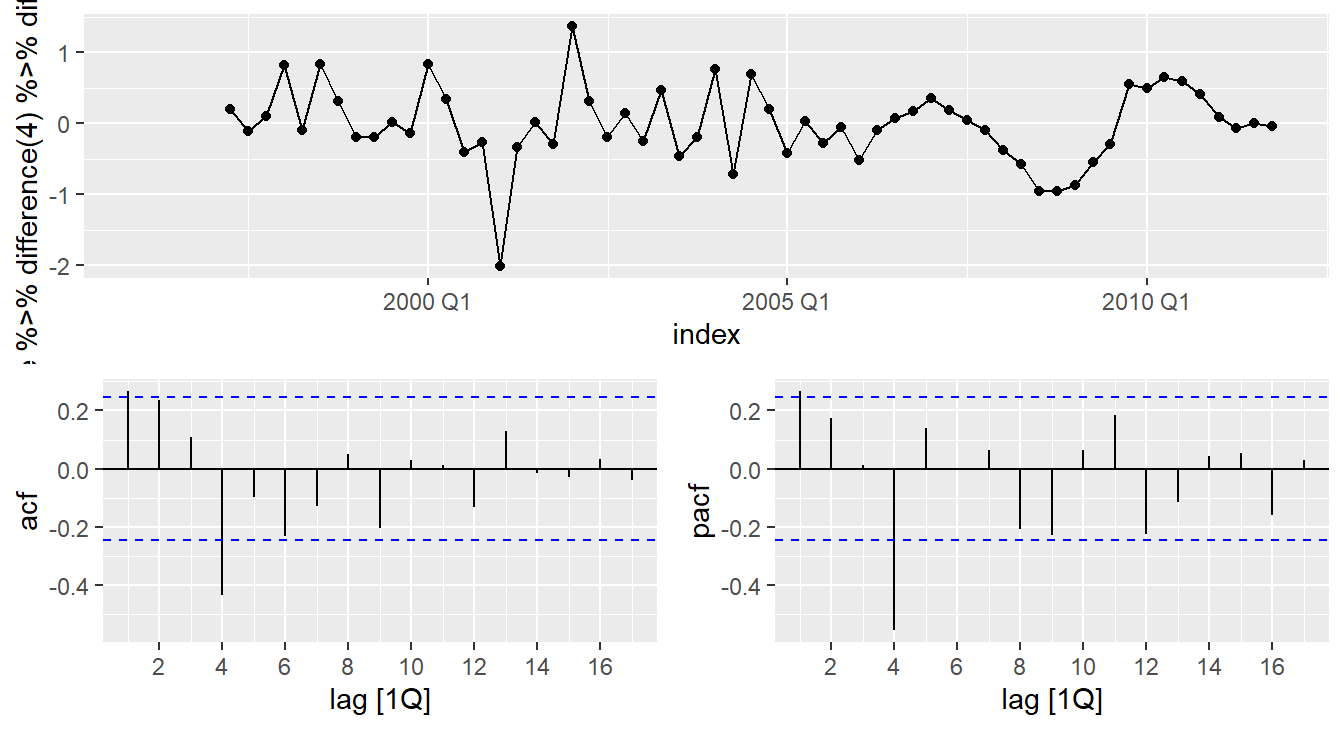
- \(d=1\) and \(D=1\) seems necessary.
- Significant spike at lag 1 in ACF suggests non-seasonal MA(1) component.
- Significant spike at lag 4 in ACF suggests seasonal MA(1) component.
- Initial candidate model: ARIMA(0,1,1)(0,1,1)\(_4\).
- We could also have started with ARIMA(1,1,0)(1,1,0)\(_4\).
fit <- eu_retail %>%
  model(arima = ARIMA(value ~ pdq(0,1,1) + PDQ(0,1,1)))
augment(fit) %>% gg_tsdisplay(.resid, plot_type = "hist")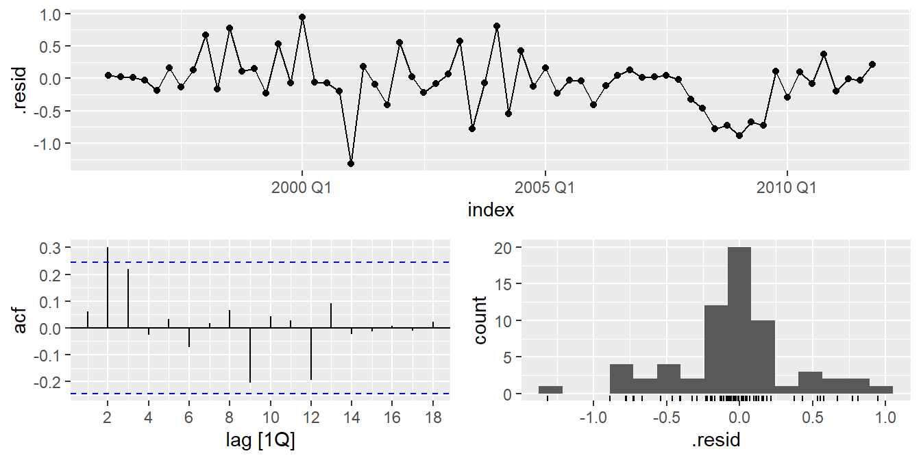
augment(fit) %>%
  features(.resid, ljung_box, lag = 8, dof = 2)
## # A tibble: 1 × 3
## .model lb_stat lb_pvalue
## <chr> <dbl> <dbl>
## 1 arima 10.7 0.0997aicc <- eu_retail %>%
model(
mdl_1 = ARIMA(value ~ pdq(0,1,1) + PDQ(0,1,1)),
mdl_2 = ARIMA(value ~ pdq(0,1,2) + PDQ(0,1,1)),
mdl_3 = ARIMA(value ~ pdq(0,1,3) + PDQ(0,1,1)),
mdl_4 = ARIMA(value ~ pdq(0,1,4) + PDQ(0,1,1))
) %>%
glance %>%
pull(AICc)- ACF and PACF of residuals show significant spikes at lag 2, and maybe lag 3.
- AICc of ARIMA(0,1,1)(0,1,1)\(_4\) model is 75.72
- AICc of ARIMA(0,1,2)(0,1,1)\(_4\) model is 74.27.
- AICc of ARIMA(0,1,3)(0,1,1)\(_4\) model is 68.39.
- AICc of ARIMA(0,1,4)(0,1,1)\(_4\) model is 70.73.
fit <- eu_retail %>%
  model(
    arima013011 = ARIMA(value ~ pdq(0,1,3) + PDQ(0,1,1))
  )
report(fit)
## Series: value
## Model: ARIMA(0,1,3)(0,1,1)[4]
##
## Coefficients:
## ma1 ma2 ma3 sma1
## 0.2630 0.3694 0.4200 -0.6636
## s.e. 0.1237 0.1255 0.1294 0.1545
##
## sigma^2 estimated as 0.156: log likelihood=-28.63
## AIC=67.26 AICc=68.39 BIC=77.65augment(fit) %>%
gg_tsdisplay(.resid, plot_type = "hist")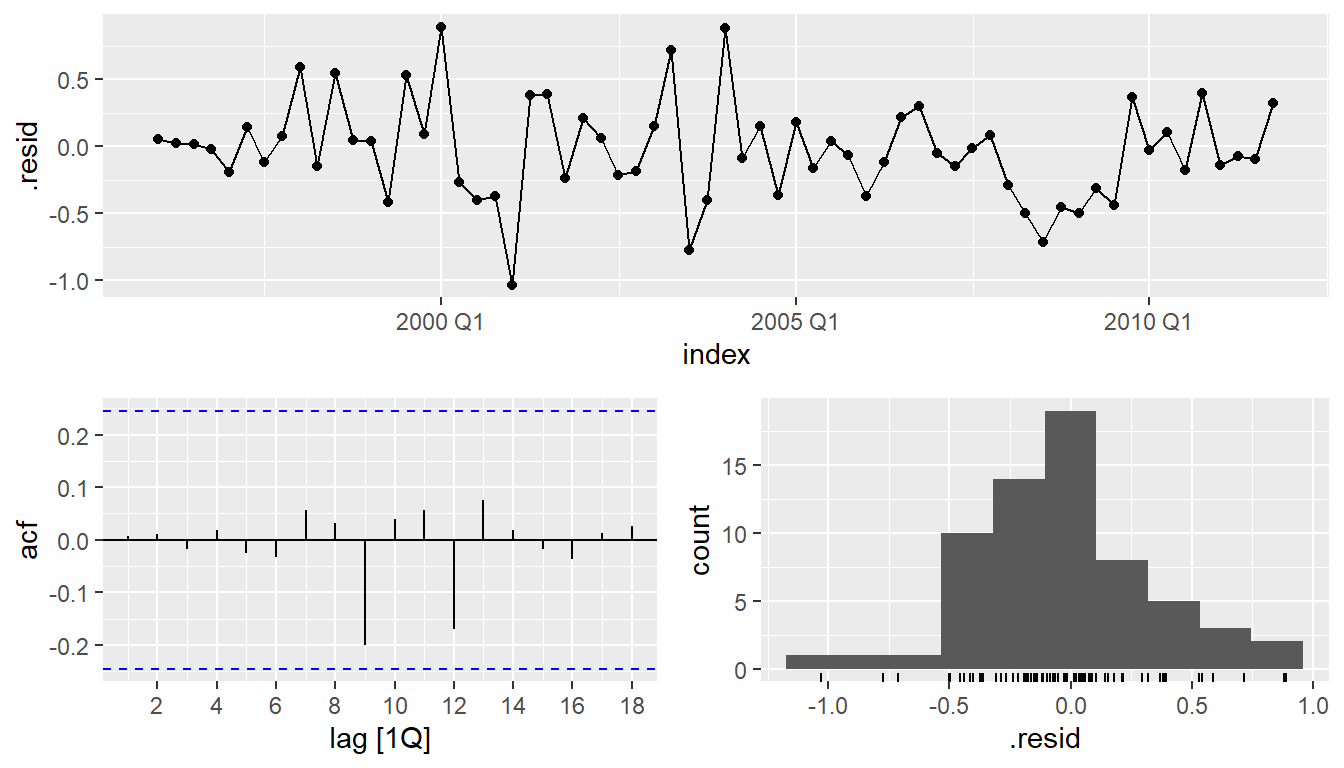
augment(fit) %>%
  features(.resid, ljung_box, lag = 8, dof = 4)
## # A tibble: 1 × 3
## .model lb_stat lb_pvalue
## <chr> <dbl> <dbl>
## 1 arima013011 0.511 0.972fit %>% forecast(h = "3 years") %>%
autoplot(eu_retail)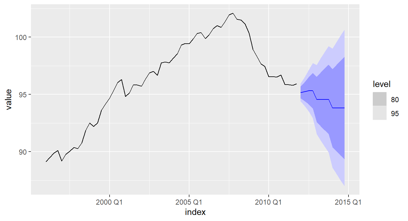
eu_retail %>% model(ARIMA(value)) %>% report()## Series: value
## Model: ARIMA(0,1,3)(0,1,1)[4]
##
## Coefficients:
## ma1 ma2 ma3 sma1
## 0.2630 0.3694 0.4200 -0.6636
## s.e. 0.1237 0.1255 0.1294 0.1545
##
## sigma^2 estimated as 0.156: log likelihood=-28.63
## AIC=67.26 AICc=68.39 BIC=77.65eu_retail %>% model(ARIMA(value, stepwise = FALSE,
approximation = FALSE)) %>% report()## Series: value
## Model: ARIMA(0,1,3)(0,1,1)[4]
##
## Coefficients:
## ma1 ma2 ma3 sma1
## 0.2630 0.3694 0.4200 -0.6636
## s.e. 0.1237 0.1255 0.1294 0.1545
##
## sigma^2 estimated as 0.156: log likelihood=-28.63
## AIC=67.26 AICc=68.39 BIC=77.65