Chapter 14 Univariate Analysis
14.1 Measurement Scales
We have two kinds of variables:
Qualitative, or Attribute, or Categorical, Variable: A variable that categorizes or describes an element of a population. Note: Arithmetic operations, such as addition and averaging, are not meaningful for data resulting from a qualitative variable.
Quantitative, or Numerical, Variable: A variable that quantifies an element of a population. Note: Arithmetic operations such as addition and averaging, are meaningful for data resulting from a quantitative variable.
Qualitative and quantitative variables may be further subdivided:
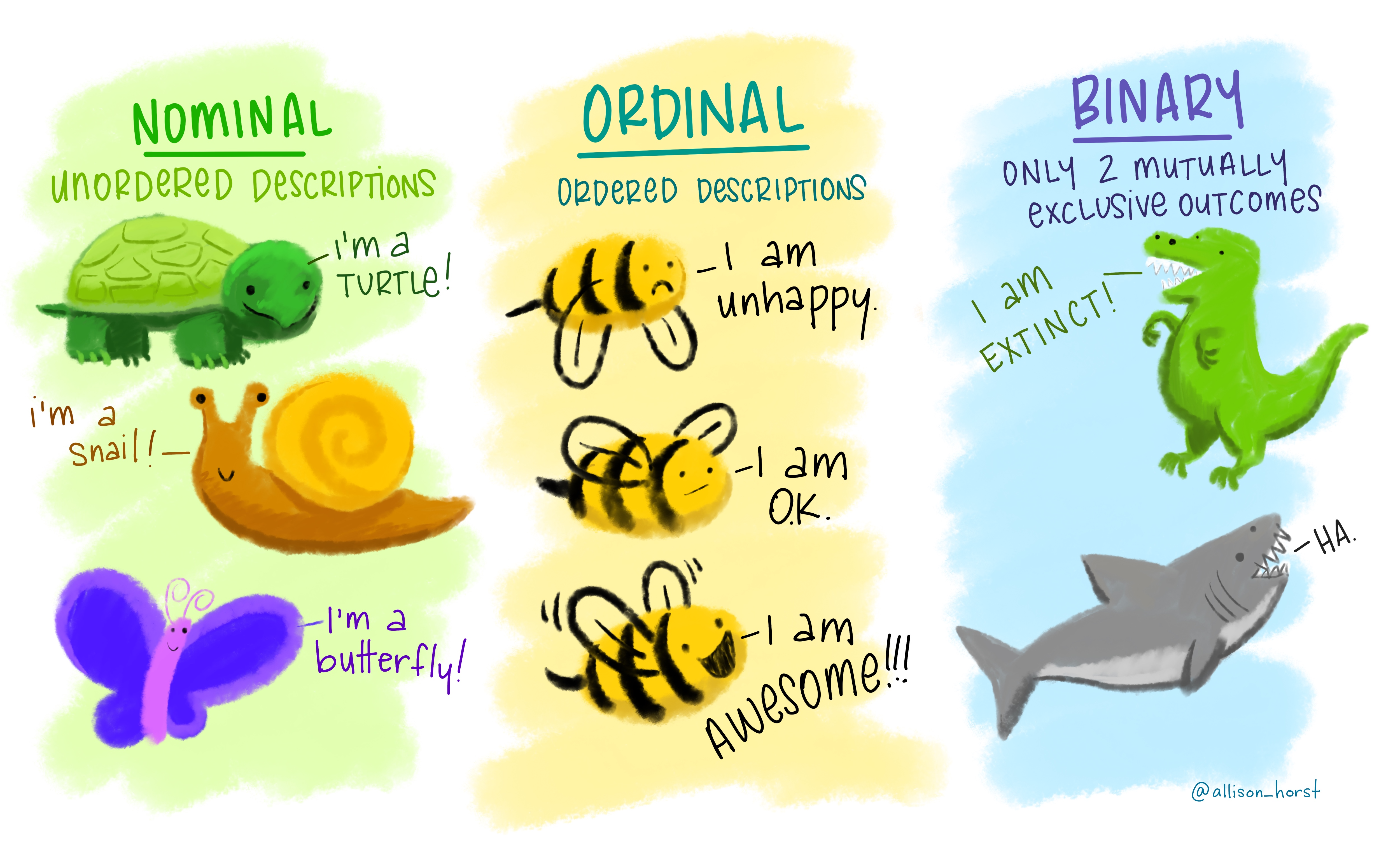
Nominal Variable: A qualitative variable that categorizes (or describes, or names) an element of a population.
Ordinal Variable: A qualitative variable that incorporates an ordered position, or ranking.
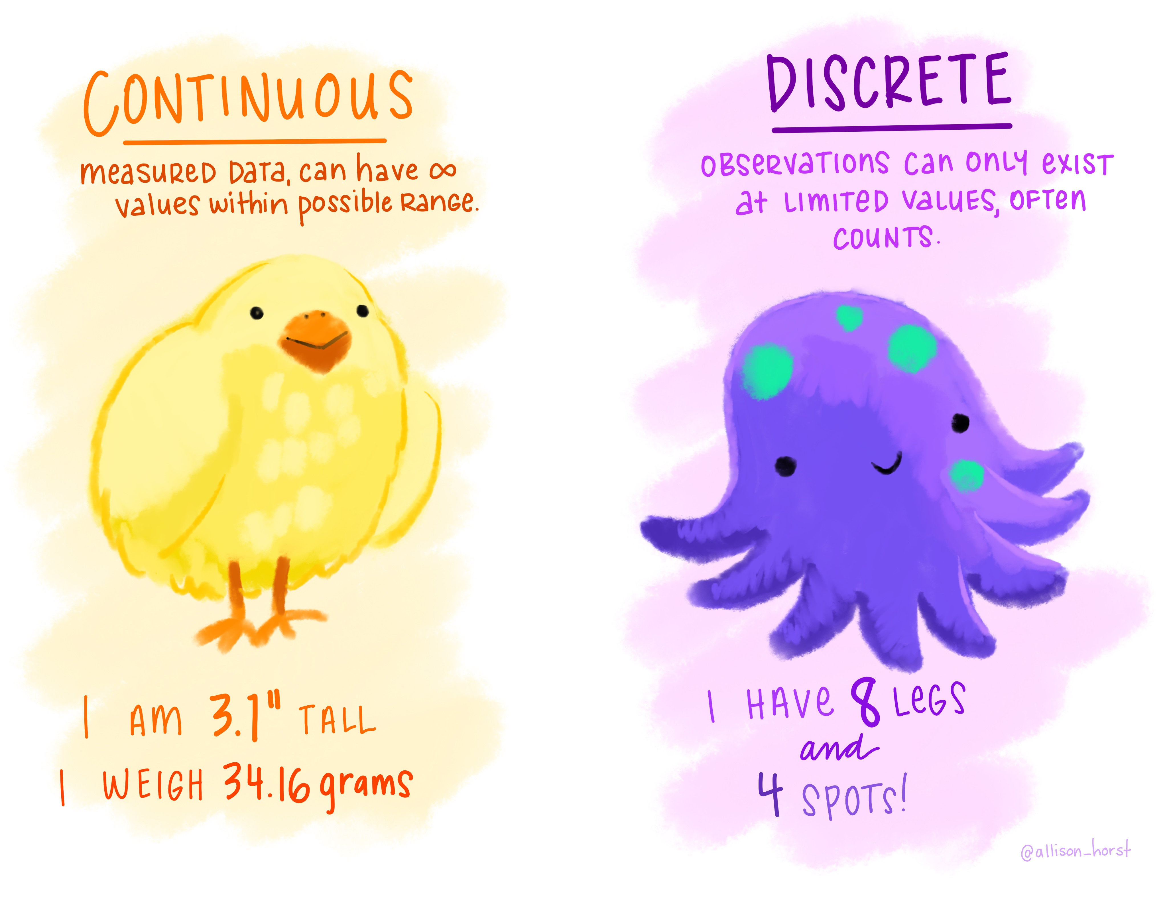
Discrete Variable: A quantitative variable that can assume a countable number of values. Intuitively, a discrete variable can assume values corresponding to isolated points along a line interval. That is, there is a gap between any two values. One example: binary variable (0-1).
Continuous Variable: A quantitative variable that can assume an uncountable number of values. Intuitively, a continuous variable can assume any value along a line interval, including every possible value between any two values.
14.2 Central Tendency
We can use many different statistics to describe the central tendency of a given distribution.
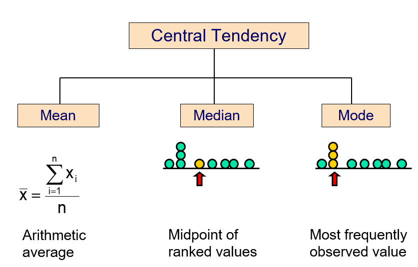
14.2.1 Arithmetic mean
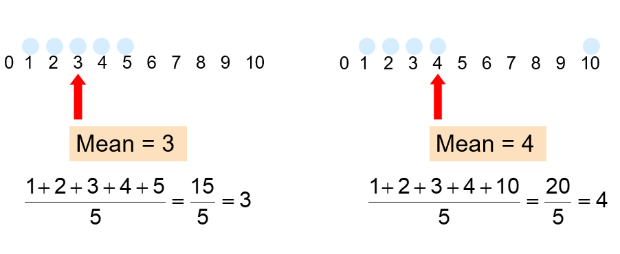
The arithmetic mean (mean) is the most common measure of central tendency.
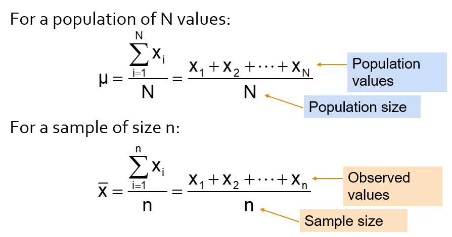
Mean = sum of values divided by the number of values, but unfortunately it is easily affected by extreme values (outliers).
- It requires at least the interval scale.
- All values are used
- It is unique
- It is easy to calculate and allow easy mathematical treatment
- The sum of the deviations from the mean is 0
- The arithmetic mean is the only measure of central tendency where the sum of the deviations of each value from the mean is zero!
- It is easily affected by extremes, such as very big or small numbers in the set (non-robust)
- For data stored in frequency tables use weighted mean!
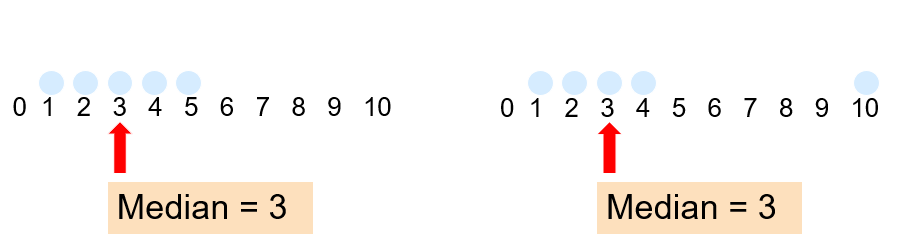
14.2.2 Median
In an ordered list, the median is the “middle” number (50% above, 50% below).
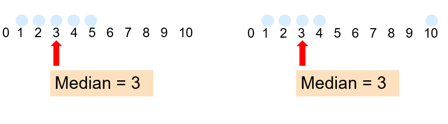
Not affected by extreme values!
- It requires at least the ordinal scale
- All values are used
- It is unique
- It is easy to calculate but does not allow easy mathematical treatment
- It is not affected by extremely large or small numbers (robust)!
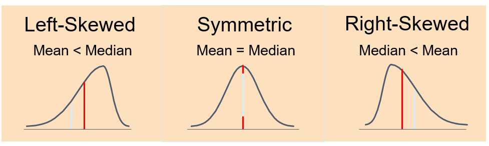
Median and mean may describe how data are distributed. Their comparison may witness of shape = if it is symmetric or skewed:
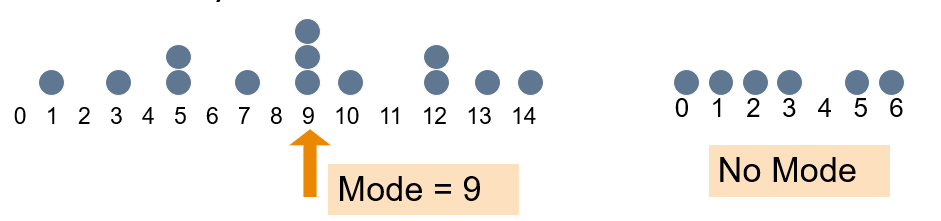
14.2.3 Mode
Mode is a measure of central tendency = the value that occurs most often. It is not affected by extreme values!
Usually used for either numerical or categorical data!
There may may be no mode!
There may be several modes!!
14.2.4 Quantiles
Quantiles are values that split sorted data or a probability distribution into equal parts. In general terms, a q-quantile divides sorted data into q parts. The most commonly used quantiles have special names:
- Quartiles (4-quantiles): Three quartiles split the data into four parts.
- Deciles (10-quantiles): Nine deciles split the data into 10 parts.
- Percentiles (100-quantiles): 99 percentiles split the data into 100 parts.
There is always one fewer quantile than there are parts created by the quantiles.
Quartiles
Quartiles split the ranked data into 4 segments with an equal number of values per segment:
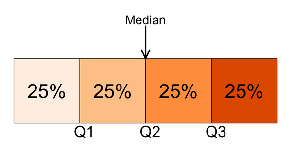
The first quartile, Q1, is the value for which 25% of the observations are smaller and 75% are larger. Q2 is the same as the median (50% are smaller, 50% are larger). Only 25% of the observations are greater than the third quartile!
Deciles
Further division of a distribution into a number of equal parts is sometimes used; the most common of these are deciles, percentiles, and fractiles.
Deciles divide the sorted data into 10 sections.
Percentiles
Percentiles divide the distribution into 100 sections
Fractiles
Instead of using a percentile we would refer to a fractile. For example, the 30th percentile is the 0.30 fractile.